Représentation et inférence de réseaux avec R et Python
State of the R
24-28/08/2020
Utilisation de Python dans rmarkdown
Pour pouvoir utiliser Python dans Rmarkdown il faut utiliser le package reticulate. On peut lui préciser le chemin de la version que l’on veut utiliser une certaine version plutôt que celle par défaut. Si une version de Python est déjà chargée, il faut relancer la session R pour que la modification soit appliqué.
library(reticulate)
use_virtualenv("r-reticulate")
reticulate::py_config()
## python: /usr/share/miniconda/envs/finistR2020/bin/python3
## libpython: /usr/share/miniconda/envs/finistR2020/lib/libpython3.8.so
## pythonhome: /usr/share/miniconda/envs/finistR2020:/usr/share/miniconda/envs/finistR2020
## version: 3.8.5 | packaged by conda-forge | (default, Aug 29 2020, 01:22:49) [GCC 7.5.0]
## numpy: /usr/share/miniconda/envs/finistR2020/lib/python3.8/site-packages/numpy
## numpy_version: 1.19.1
##
## python versions found:
## /usr/share/miniconda/envs/finistR2020/bin/python3
## /usr/bin/python3
## /usr/bin/pythonIl suffit alors de créer un chunk avec python comme langage. Tous les objets R de l’environnement sont accessible via la commande r..
x = 2
print(x)
## 2r.x = xDans un chunk R, les objets python sont accessible avec la commande py$.
x <- py$x
y <- x**2
print(y)
## [1] 4typeof(y)## [1] "double"Il faut faire attention à la transformation automatique des types de R vers python, ce dernier étant plus pointilleux que R la dessus.
z = [i**2 for i in range(int(r.y))]

print(z)
## [0, 1, 4, 9]Utilisation de la librarie graph_tool
graph_tool est une librairie python pour analyser des réseaux développer par T. Peixoto. Elle permet entre autre de faire des visualisations interactive de graphes et est également très réputée pour ces implémentations du SBM et du degree corrected SBM.
library(sbm)
library(igraph)
library(tidyverse)
import graph_tool.all as gt
import matplotlib.pyplot as plt
import numpy as np
import math
import timeg = gt.collection.data["football"]
print(g)## <Graph object, undirected, with 115 vertices and 613 edges, 4 internal vertex properties, 2 internal graph properties, at 0x7fe89413f190>state = gt.minimize_blockmodel_dl(g)
m = state.get_matrix()Les plots matplotlib sortent très bien dans le notebook, mais ce n’est pas le cas des plots interactifs. Ceux-ci ouvrent une fenêtre python interactive et bloquent la compilation du document.
plt.matshow(m.todense())Si l’on décide de sortir un plot inline, la fenêtre virtuelle ne s’ouvre pas et l’on récupère juste l’adresse mémoire du graph stocker. Il faut sauver dans un fichier et insérer “à la main”
pv = None
for i in range(1000):
     ret = state.mcmc_sweep(niter=10)
     pv = state.collect_vertex_marginals(pv)
gt.mf_entropy(g, pv)
## 3.101857666590992p = gt.graph_draw(g, pos=g.vp["pos"], vertex_shape="pie",
vertex_pie_fractions=pv, inline= True, output = "img/hier.png")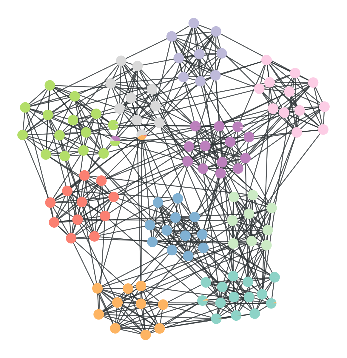
plot hierarchique
On obtient des représentations graphiques sur des graph assez gros (1500 noeuds) rapidement.
g = gt.price_network(1500)
deg = g.degree_property_map("in")
deg.a = 4 * (np.sqrt(deg.a) * 0.5 + 0.4)
ebet = gt.betweenness(g)[1]
ebet.a /= ebet.a.max() / 10.
eorder = ebet.copy()
eorder.a *= -1
pos = gt.sfdp_layout(g)
control = g.new_edge_property("vector<double>")
for e in g.edges():
    d = np.sqrt(sum((pos[e.source()].a - pos[e.target()].a) ** 2)) / 5
    control[e] = [0.3, d, 0.7, d]
gt.graph_draw(g, pos=pos, vertex_size=deg, vertex_fill_color=deg, vorder=deg,
              edge_color=ebet, eorder=eorder, edge_pen_width=ebet,
              edge_control_points=control, # some curvy edges
              output="img/graph-draw.png")
## <VertexPropertyMap object with value type 'vector<double>', for Graph 0x7fe892d59790, at 0x7fe892d50970>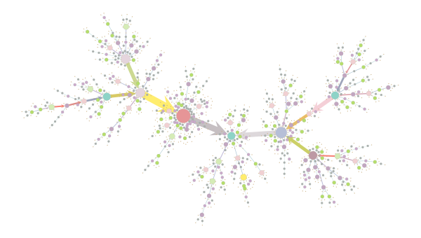
graph1500
Et l’on peut également sortir des plots interactifs avec graphviz.
g = gt.price_network(1500)
deg = g.degree_property_map("in")
deg.a = 2 * (np.sqrt(deg.a) * 0.5 + 0.4)
ebet = gt.betweenness(g)[1]
#gt.graphviz_draw(g, vcolor=deg, vorder=deg, elen=10,
#                 ecolor=ebet, eorder=ebet, )#, output="graphviz-draw.pdf")
g = gt.price_network(3000)
pos = gt.sfdp_layout(g)
gt.graph_draw(g, pos=pos)#, output="graph-draw-sfdp.pdf")g = gt.collection.data["netscience"]
g = gt.GraphView(g, vfilt=gt.label_largest_component(g))
g.purge_vertices()
state = gt.minimize_nested_blockmodel_dl(g, deg_corr=True)
t = gt.get_hierarchy_tree(state)[0]
tpos = pos = gt.radial_tree_layout(t, t.vertex(t.num_vertices() - 1), weighted=True)
cts = gt.get_hierarchy_control_points(g, t, tpos)
pos = g.own_property(tpos)
b = state.levels[0].b
shape = b.copy()
shape.a %= 14
gt.graph_draw(g, pos=pos, vertex_fill_color=b, vertex_shape=shape,
edge_control_points=cts,
edge_color=[0, 0, 0, 0.3], vertex_anchor=0)#, output="netscience_nested_mdl.pdf")Un essaie de plot hiérarchique:
g = gt.collection.data["celegansneural"]
state = gt.minimize_nested_blockmodel_dl(g, deg_corr=True)
gt.draw_hierarchy(state, output="img/celegansneural_hier.png")
## (<VertexPropertyMap object with value type 'vector<double>', for Graph 0x7fe892d326a0, at 0x7fe892cecac0>, <Graph object, directed, with 317 vertices and 316 edges, at 0x7fe892d4cc40>, <VertexPropertyMap object with value type 'vector<double>', for Graph 0x7fe892d4cc40, at 0x7fe892d59d90>)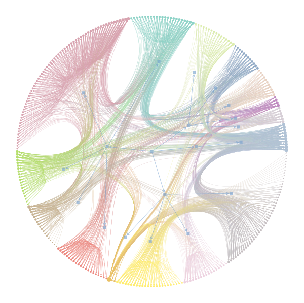
plot hierarchique
Si l’on fit un sbm sur un graph, l’autoplot sur l’état des blocks du graphe se fait automatiquement.
t0 = time.time()
g = gt.collection.data["polbooks"]

state = gt.minimize_blockmodel_dl(g , deg_corr=False)
for i in range(10):
    s = gt.minimize_blockmodel_dl(g , deg_corr=False)
    if s.entropy() < state.entropy():
        state = s

t = t0 - time.time()
print(t)
## -16.440711975097656state.entropy()## 1321.9479136333077state.draw(pos=g.vp["pos"], vertex_shape=state.get_blocks(), output="img/polbooks_blocks_mdl.svg")## <VertexPropertyMap object with value type 'vector<double>', for Graph 0x7fe892cec760, at 0x7fe892cecc70>
Image graph tools
Passe de python à R
On peut passer le réseau via la matrice d’adjacence de python à R, mais on aimerait mieux sortir un objet graphml qui est bien lu par igraph.
Malheureusement, cela ne fonctionne pas. Toutes les méthodes de graph_tool sur les noeuds et les arêtes renvoient des itérateurs. Il est nécessaire de les transformer en vecteur avec de les utiliser en R.
blocks = [b for b in state.get_blocks()]
A = gt.adjacency(g)
## g.save(file_name= "/home/stc/Documents/StateOfTheR/FinistR2020/graph_gt.graphml", fmt="graphml")py$blocks + 1## [1] 1 1 6 2 6 1 1 6 2 1 2 2 2 2 1 3 3 3 1 3 1 3 1 3 1 1 1 3 4 1 5 5 3 3 3 3 3
## [38] 3 3 3 2 3 3 3 3 1 3 2 1 6 1 6 6 1 3 3 3 1 6 4 4 4 4 4 6 6 5 6 6 6 4 5 5 5
## [75] 5 5 5 4 4 4 4 4 4 4 5 6 5 4 4 4 4 4 4 4 4 4 4 4 4 5 5 4 4 6 6A <- as.matrix(py$A)
isSymmetric(A)## [1] TRUEmy_sbm <- blockmodels::BM_bernoulli("SBM_sym", A, verbosity = 0, plotting = "")t0 <- Sys.time()
my_sbm$estimate()t <- t0 - Sys.time()
t## Time difference of -6.823365 secsaricode::ARI(c1 = py$blocks +1, c2 = my_sbm$memberships[[5]]$map()$C)## [1] 0.7586591my_sbm$memberships[[5]]$map()$C## [1] 3 3 3 2 3 3 3 3 2 2 2 2 2 2 1 1 1 1 1 1 1 1 1 1 1 1 1 1 4 3 5 5 1 1 1 1 1
## [38] 1 1 1 2 1 1 1 1 1 1 2 1 3 1 3 3 1 1 1 1 1 3 4 4 4 4 4 3 3 5 3 3 3 4 5 5 5
## [75] 5 5 5 4 4 4 4 4 4 4 5 3 5 4 4 4 4 4 4 4 4 4 4 4 4 5 5 4 4 3 3py$blocks +1## [1] 1 1 6 2 6 1 1 6 2 1 2 2 2 2 1 3 3 3 1 3 1 3 1 3 1 1 1 3 4 1 5 5 3 3 3 3 3
## [38] 3 3 3 2 3 3 3 3 1 3 2 1 6 1 6 6 1 3 3 3 1 6 4 4 4 4 4 6 6 5 6 6 6 4 5 5 5
## [75] 5 5 5 4 4 4 4 4 4 4 5 6 5 4 4 4 4 4 4 4 4 4 4 4 4 5 5 4 4 6 6Les clustering obtenus par graph-tool et sbm (blockmodels) sont très proche pour le sbm simple.
igraph::graph_from_adjacency_matrix(
  A, mode = "directed") %>% igraph::write_graph(file = "graph_test.graphml", format = "graphml")
gr = gt.load_graph(file_name="~/Documents/StateOfTheR/FinistR2020/graph_test.graphml", fmt="graphml")gr.set_directed = False
gt.minimize_blockmodel_dl(gr, deg_corr=False)Reste à faire
- Trouver une meilleur méthode pour passer un objet de type graph de
pythonversR. Une solution serait peut-être d’utiliser le moduleigraphdepython. - Est-il possible de capturer une fenêtre interactive
pythonpour la mettre dans la sortie html durmarkdown?