PLN version Python

PLN with Pytorch

Comme vous pourrez le constater, les syntaxtes {torch} et Pytorch sont très proches.

Préliminaires

On charge le jeu de données oaks contenu dans le package python pyPLNmodels

import pyPLNmodels
import numpy as np
import matplotlib.pyplot as plt
from pyPLNmodels.models import PlnPCAcollection, Pln
from pyPLNmodels.oaks import load_oaks
oaks = load_oaks()
Y = oaks['counts']
O = np.log(oaks['offsets'])
X = np.ones([Y.shape[0],1])

Pour référence, on optimise avec le package dédié (qui utilise pytorch et l’optimiseur Rprop.

pln = Pln.from_formula("counts ~ 1 ", data = oaks, take_log_offsets = True)
%timeit pln.fit()

Fitting a Pln model with full covariance model.
Initialization ...
Initialization finished
Tolerance 0.001 reached in 264 iterations
Fitting a Pln model with full covariance model.
Tolerance 0.001 reached in 265 iterations
Fitting a Pln model with full covariance model.
Tolerance 0.001 reached in 299 iterations
Fitting a Pln model with full covariance model.
Tolerance 0.001 reached in 300 iterations
Fitting a Pln model with full covariance model.
Tolerance 0.001 reached in 332 iterations
Fitting a Pln model with full covariance model.
Tolerance 0.001 reached in 347 iterations
Fitting a Pln model with full covariance model.
Tolerance 0.001 reached in 362 iterations
Fitting a Pln model with full covariance model.
Tolerance 0.001 reached in 371 iterations
The slowest run took 36.93 times longer than the fastest. This could mean that an intermediate result is being cached.
38.9 ms ± 32.6 ms per loop (mean ± std. dev. of 7 runs, 1 loop each)

Implémentation simple en Pytorch

import torch
import numpy as np
import math

def _log_stirling(integer: torch.Tensor) -> torch.Tensor:
    integer_ = integer + (integer == 0)  # Replace 0 with 1 since 0! = 1!
    return torch.log(torch.sqrt(2 * np.pi * integer_)) + integer_ * torch.log(integer_ / math.exp(1))

class PLN() :
    Y : torch.Tensor
    O : torch.Tensor
    X : torch.Tensor
    n : int
    p : int
    d : int
    M : torch.Tensor
    S : torch.Tensor
    B : torch.Tensor
    Sigma : torch.Tensor
    Omega : torch.Tensor
    ELBO_list : list

      ## Constructor
    def __init__(self, Y: np.array, O: np.array, X: np.array) : 
        self.Y = torch.tensor(Y)
        self.O = torch.tensor(O)
        self.X = torch.tensor(X)
        self.n, self.p = Y.shape
        self.d = X.shape[1]
        ## Variational parameters
        self.M = torch.full(Y.shape, 0.0, requires_grad = True)
        self.S = torch.full(Y.shape, 1.0, requires_grad = True)
        ## Model parameters
        self.B = torch.zeros(self.d, self.p, requires_grad = True)
        self.Sigma = torch.eye(self.p)
        self.Omega = torch.eye(self.p)

    def get_Sigma(self) :
      return 1/self.n * (self.M.T @ self.M + torch.diag(torch.sum(self.S**2, dim = 0)))

    def get_ELBO(self): 
      S2 = torch.square(self.S)
      XB = self.X @ self.B
      A = torch.exp(self.O + self.M + XB + S2/2)

      elbo = self.n/2 * torch.logdet(self.Omega) +  torch.sum(- A + self.Y * (self.O + self.M + XB) + .5 * torch.log(S2)) - .5 * torch.trace(self.M.T @ self.M + torch.diag(torch.sum(S2, dim = 0)) @ self.Omega) + .5 * self.n * self.p  - torch.sum(_log_stirling(self.Y))
      return elbo

    def fit(self, N_iter, lr, tol = 1e-8) :
      self.ELBO = np.zeros(N_iter)
      optimizer = torch.optim.Rprop([self.B, self.M, self.S], lr = lr)
      objective0 = np.infty
      for i in range(N_iter):
        ## reinitialize gradients
        optimizer.zero_grad()

        ## compute current ELBO
        loss = - self.get_ELBO()

        ## backward propagation and optimization
        loss.backward()
        optimizer.step()

        ## update parameters with close form
        self.Sigma = self.get_Sigma()
        self.Omega = torch.inverse(self.Sigma)

        objective = -loss.item()
        self.ELBO[i] = objective
        
        if (abs(objective0 - objective)/abs(objective) < tol):
          self.ELBO = self.ELBO[0:i]
          break
        else:
          objective0 = objective

Évaluation du temps de calcul

Testons notre implémentation simple de PLN utilisant:

myPLN = PLN(Y, O, X)
%timeit myPLN.fit(50, lr = 0.1, tol = 1e-8)
plt.plot(np.log(-myPLN.ELBO))

180 ms ± 5.77 ms per loop (mean ± std. dev. of 7 runs, 10 loops each)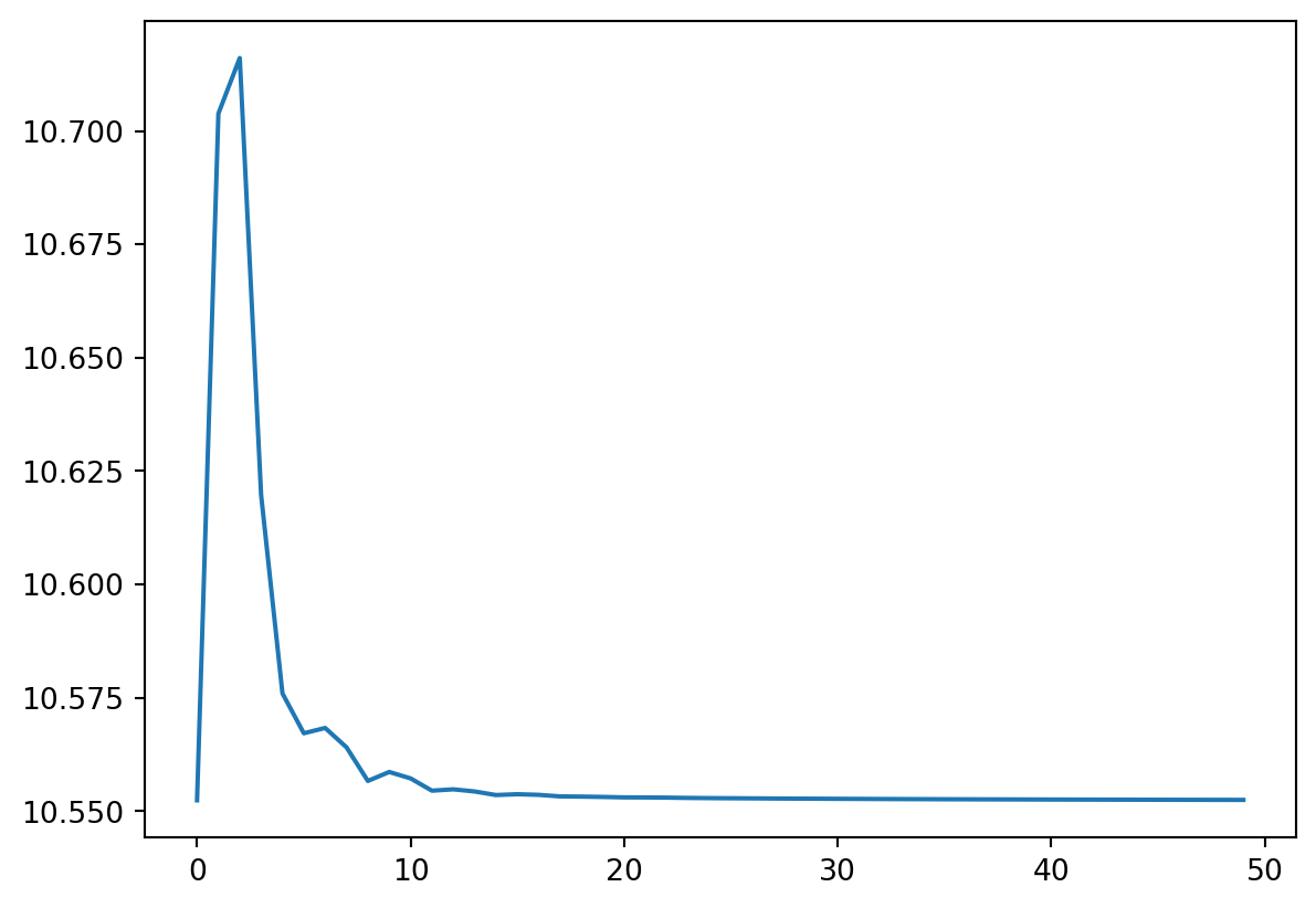

```