library(tidyverse)
library(rvest)
theme_set(theme_bw())
df <-
  "https://fr.wikipedia.org/wiki/Liste_des_pays_par_population" %>%
  read_html() %>%
  html_node('table') %>%
  html_table() %>%
  as_tibble()
df
## # A tibble: 204 x 6
##    Rang  `Pays ou territo… `Population[Note…  Date Source Commentaires
##    <chr> <chr>             <chr>             <int> <chr>  <chr>
##  1 1     Chine             1 415 045 928      2018 Offic… Pays le plus pe…
##  2 2     Inde              1 355 621 800      2018 Offic… Pays le plus pe…
##  3 •     Union européenne  512 596 403        2018 Offic… L'Union europée…
##  4 3     États-Unis        328 286 400        2018 Offic… Pays le plus pe…
##  5 4     Indonésie         266 471 000        2018 Offic… Archipel le plu…
##  6 5     Pakistan          207 774 520        2017 Offic… ""
##  7 6     Brésil            207 096 196        2017 Offic… Pays le plus pe…
##  8 7     Nigeria           190 632 261        2017 CIA W… Pays le plus pe…
##  9 8     Bangladesh        160 339 154        2016 Offic… ""
## 10 9     Russie            146 544 710        2016 Offic… La population r…
## # ... with 194 more rows
pop <- pull(df, `Population[Note 2]`)
head(pop)
## [1] "1 415 045 928" "1 355 621 800" "512 596 403"   "328 286 400"
## [5] "266 471 000"   "207 774 520"
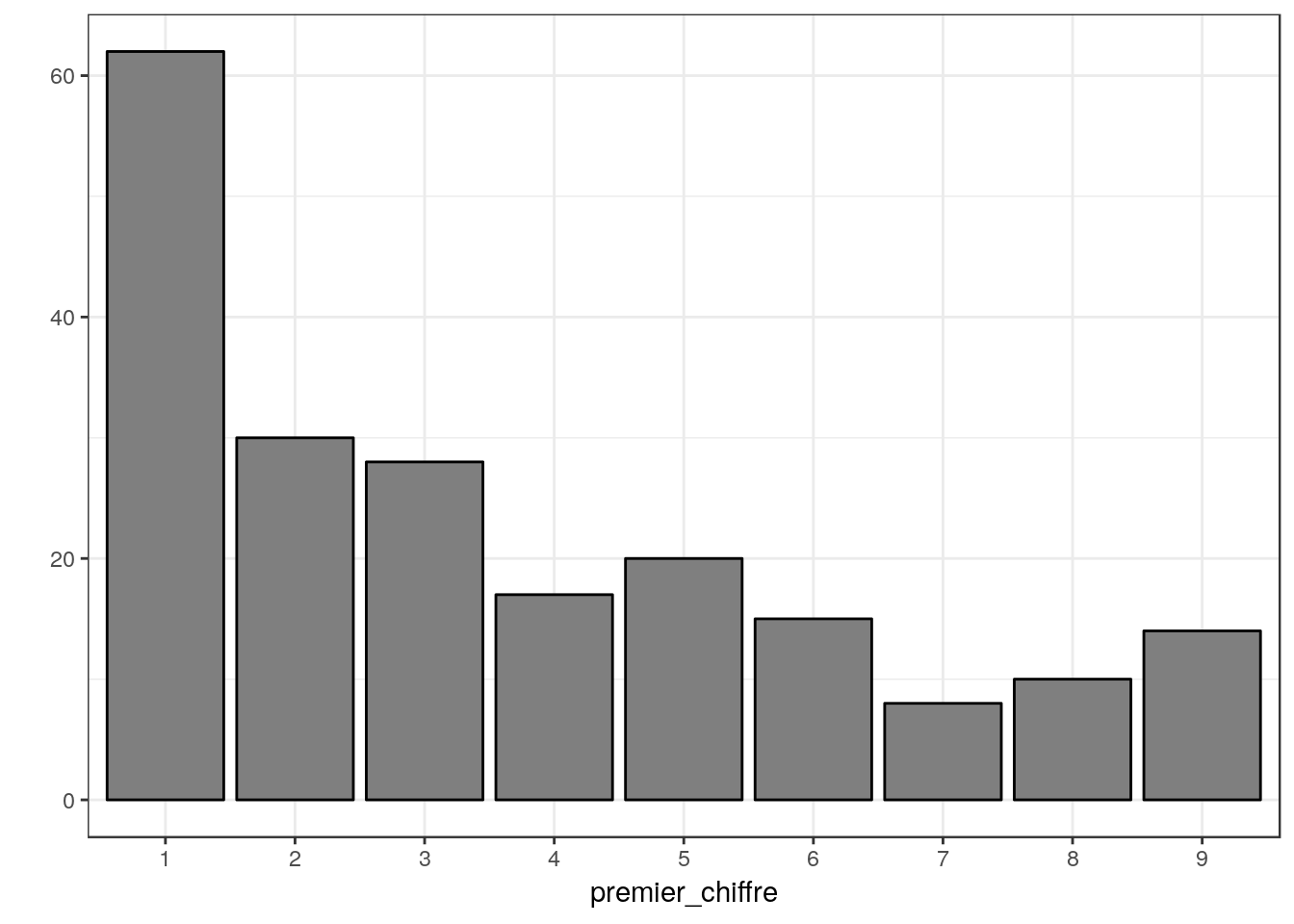
premier_chiffre <- str_sub(pop, 1, 1)
head(premier_chiffre)
## [1] "1" "1" "5" "3" "2" "2"
qplot(premier_chiffre) + geom_bar(fill = "grey50", color = "black")
frequences <-
  tibble(premier_chiffre) %>%
  group_by(premier_chiffre) %>%
  summarise(eff_obs = n()) %>%
  mutate(freq_obs = eff_obs/sum(eff_obs)) %>%
  mutate(freq_unif = 1/9,
         freq_benford = c(0.301,    0.176,  0.125,  0.097, 0.079,   0.067, 0.058,   0.051, 0.046))
frequences
## # A tibble: 9 x 5
##   premier_chiffre eff_obs freq_obs freq_unif freq_benford
##   <chr>             <int>    <dbl>     <dbl>        <dbl>
## 1 1                    62   0.304      0.111        0.301
## 2 2                    30   0.147      0.111        0.176
## 3 3                    28   0.137      0.111        0.125
## 4 4                    17   0.0833     0.111        0.097
## 5 5                    20   0.0980     0.111        0.079
## 6 6                    15   0.0735     0.111        0.067
## 7 7                     8   0.0392     0.111        0.058
## 8 8                    10   0.0490     0.111        0.051
## 9 9                    14   0.0686     0.111        0.046
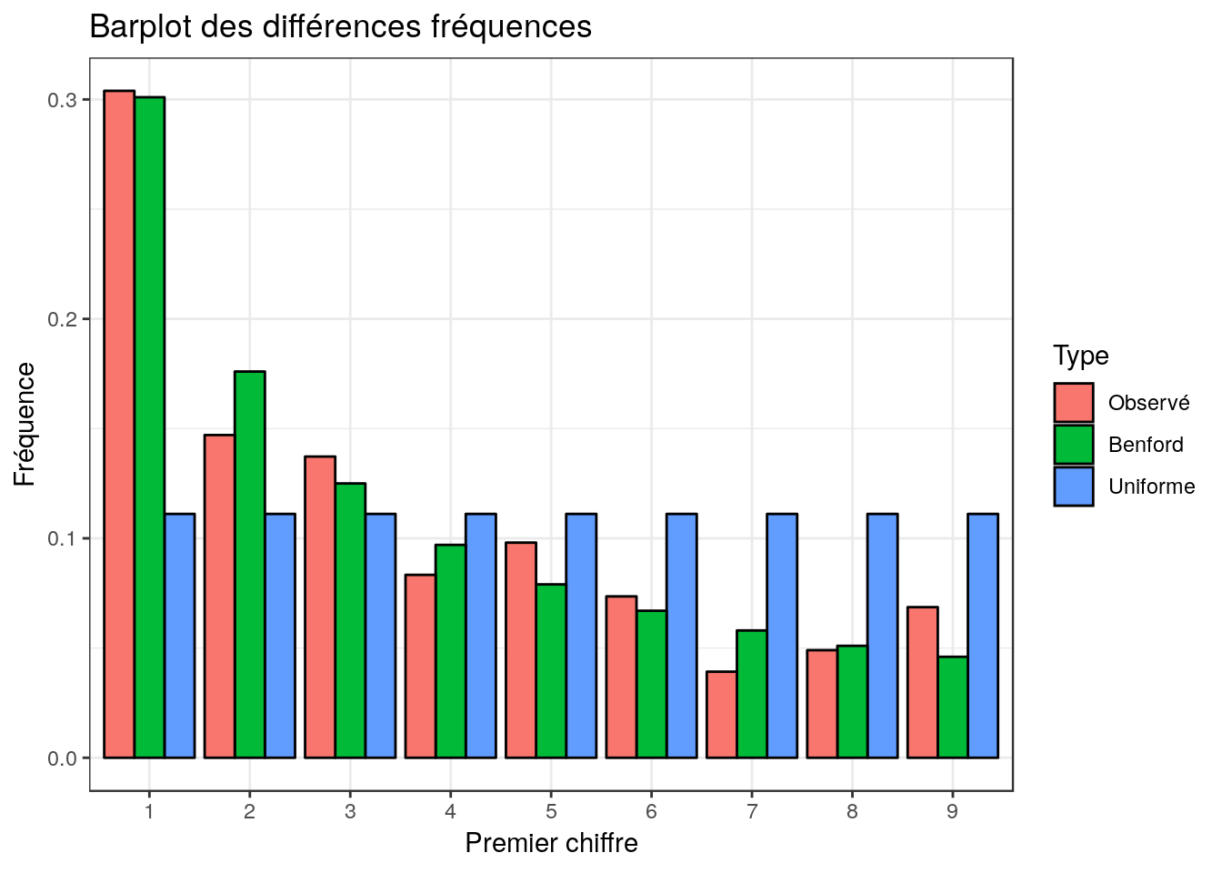
frequences %>%
  select(premier_chiffre, freq_obs, freq_unif, freq_benford) %>%
  gather(-premier_chiffre, key = type, value = freq) %>%
  mutate(type = factor(type,
                       levels = c("freq_obs", "freq_benford", "freq_unif"),
                       labels = c("Observé", "Benford", "Uniforme"))) %>%
  print() %>%
  ggplot() +
  aes(x = premier_chiffre, y = freq, fill = type) +
  geom_col(position = "dodge", color = "black") +
  labs(x = "Premier chiffre", y = "Fréquence",
       fill = "Type", title = "Barplot des différences fréquences")
## # A tibble: 27 x 3
##    premier_chiffre type       freq
##    <chr>           <fct>     <dbl>
##  1 1               Observé  0.304
##  2 2               Observé  0.147
##  3 3               Observé  0.137
##  4 4               Observé  0.0833
##  5 5               Observé  0.0980
##  6 6               Observé  0.0735
##  7 7               Observé  0.0392
##  8 8               Observé  0.0490
##  9 9               Observé  0.0686
## 10 1               Uniforme 0.111
## # ... with 17 more rows