Objectif

Le but de ce tutoriel est de faire un TP de modèle linéaire en python, en retrouvant tout les sorties de la fonction lm usuelle

Python depuis `rstudio`

Package `reticulate`

On peut appeler python depuis Rstudio grâce au package reticulate.

library(reticulate)

Après avoir chargé ce package, toute instruction en python sera reconnue comme tel dans la console!

Installation des librairies python depuis `R`

Pour installer les librairies, on utilisera les instructions R suivantes:

# Run only once
install_miniconda() ## pour installer miniconda

## [1] "/github/home/.local/share/r-miniconda"

py_install("pandas") # Pour la manipulation de données
py_install("numpy") # Librairie scientifique
py_install("scipy") # Librairie scientifique
py_install("scikit-learn") # Librairie de machine learning
py_install("seaborn") # Librairie graphique
py_install("statsmodels") # Librairie de modèles statistiques
py_install("yellowbrick") # Librairie graphique

Importation des modules python

Ceci étant fait, on peut ne plus faire que du python!

import pandas as pd
import seaborn as sns
import matplotlib.pyplot as plt
import sklearn as sk
import numpy as np
import statsmodels.api as sm
import statsmodels.formula.api as smf
import scipy.stats as stats

from yellowbrick.datasets import load_concrete
from yellowbrick.regressor import ResidualsPlot
from yellowbrick.regressor import CooksDistance

from sklearn.linear_model import LinearRegression
from sklearn import datasets

plt.style.use('ggplot') # if you are an R user and want to feel at home

from statsmodels.graphics.gofplots import ProbPlot

Importation, manipulation et description des données

On utilisera la library de python pandas pour manipuler les données

Import

Ensuite, on importe la librairie, et on charge les données, à la manière de read.table.

import pandas
bats = pandas.read_csv("bats.csv", # Nom du fichier 
                          sep = ";", # Separateur de champs
                          skiprows = 3, # On ignore les 3 premieres lignes 
                          header = 0) # La premiere ligne correspond au nom de colonnes
print(bats)

##                      Species  Diet Clade  ...    AUD     MOB     HIP
## 0    Rousettus  aegyptiacus      1     I  ...   9.88  105.77  125.97
## 1        Epomops  franqueti      1     I  ...  10.44  107.80  159.80
## 2       Eonycteris  spelaea      1     I  ...   5.48   67.00   97.70
## 3        Cynopterus  sphinx      1     I  ...   4.77   65.27   95.40
## 4      Dobsonia  praedatrix      1     I  ...   7.09  213.43  233.30
## ..                       ...   ...   ...  ...    ...     ...     ...
## 58            Coleura  afra      3    IV  ...   4.08    3.98   12.40
## 59   Taphozous  saccolaimus      3    IV  ...   9.65   10.92   26.38
## 60      Kerivoula  papilosa      3    IV  ...   4.47    2.52   19.02
## 61           Myotis  myotis      3    IV  ...   7.50    5.23   16.24
## 62      Miniopterus  medius      3    IV  ...   4.77    5.31   17.28
## 
## [63 rows x 8 columns]

Description

# En-tete des donnees
bats.head()
# Dimension

##                     Species  Diet Clade    BOW      BRW    AUD     MOB     HIP
## 0   Rousettus  aegyptiacus      1     I  136.3  2070.00   9.88  105.77  125.97
## 1       Epomops  franqueti      1     I  120.0  2210.00  10.44  107.80  159.80
## 2      Eonycteris  spelaea      1     I   58.7  1310.00   5.48   67.00   97.70
## 3       Cynopterus  sphinx      1     I   48.3  1184.33   4.77   65.27   95.40
## 4     Dobsonia  praedatrix      1     I  184.0  3028.00   7.09  213.43  233.30

bats.shape
# Type des colonnes

## (63, 8)

bats.dtypes

## Species     object
## Diet         int64
## Clade       object
## BOW        float64
## BRW        float64
## AUD        float64
## MOB        float64
## HIP        float64
## dtype: object

bats.info()

## <class 'pandas.core.frame.DataFrame'>
## RangeIndex: 63 entries, 0 to 62
## Data columns (total 8 columns):
##  #   Column   Non-Null Count  Dtype  
## ---  ------   --------------  -----  
##  0   Species  63 non-null     object 
##  1   Diet     63 non-null     int64  
##  2   Clade    63 non-null     object 
##  3   BOW      63 non-null     float64
##  4   BRW      63 non-null     float64
##  5   AUD      63 non-null     float64
##  6   MOB      63 non-null     float64
##  7   HIP      63 non-null     float64
## dtypes: float64(5), int64(1), object(2)
## memory usage: 4.1+ KB

Changement de type d’une colonne

Description d’une colonne facteur du data.frame:

bats["Diet"] = bats["Diet"].apply(str) # Transformation de float a string
bats.Diet.describe() # Quelques statistiques

## count     63
## unique     4
## top        1
## freq      29
## Name: Diet, dtype: object

bats["Diet"].value_counts() # Comptage des occurences

## 1    29
## 3    27
## 2     5
## 4     2
## Name: Diet, dtype: int64

Première figure

plt.figure() # On specifie l'ouverture d'une figure
# Toutes les instructions suivantes se superposeront

bats.plot(x ='BOW', y = 'BRW', kind ="scatter", 
                 figsize = [8,6],
                 color ="b", alpha = 0.3, 
                fontsize = 14)

## <AxesSubplot:xlabel='BOW', ylabel='BRW'>

plt.title("BRW vs. BOW", 
          fontsize = 24, color="darkred")

## Text(0.5, 1.0, 'BRW vs. BOW')

plt.xlabel("Body weight", fontsize = 18)

## Text(0.5, 0, 'Body weight')

plt.ylabel("Brain weight", fontsize = 18)

## Text(0, 0.5, 'Brain weight')

plt.show() # On montre la figure

## findfont: Font family ['sans-serif'] not found. Falling back to DejaVu Sans.
## findfont: Font family ['sans-serif'] not found. Falling back to DejaVu Sans.
## findfont: Font family ['sans-serif'] not found. Falling back to DejaVu Sans.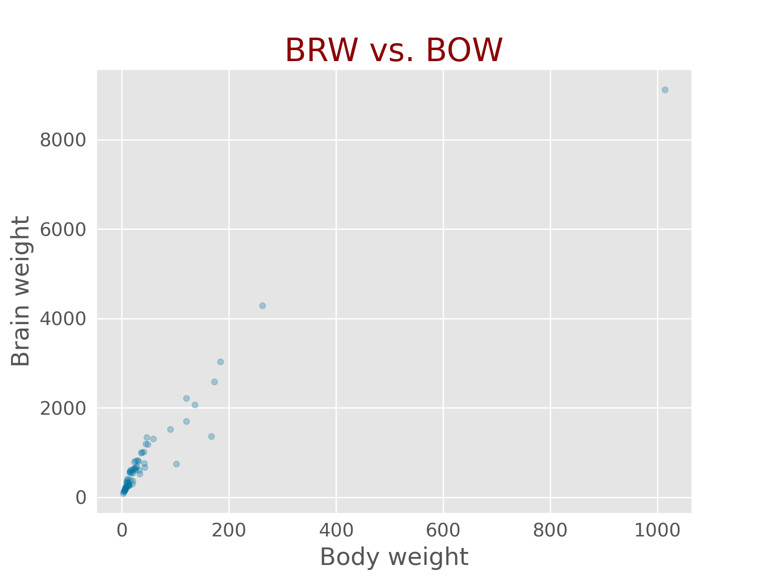

Selection logique

Pour extraire une sous partie des données, on peut utiliser la sélection par un vecteur logique.

# bats.Diet recupere la colonne Diet dans bats
condition_phyto = bats.Diet == '1' # Une colonne de condition
condition_BOW = bats.BOW < 400 # Outlier
batsphyto = bats[condition_phyto & condition_BOW]
batsphyto

##                         Species Diet Clade  ...    AUD     MOB     HIP
## 0       Rousettus  aegyptiacus     1     I  ...   9.88  105.77  125.97
## 1           Epomops  franqueti     1     I  ...  10.44  107.80  159.80
## 2          Eonycteris  spelaea     1     I  ...   5.48   67.00   97.70
## 3           Cynopterus  sphinx     1     I  ...   4.77   65.27   95.40
## 4         Dobsonia  praedatrix     1     I  ...   7.09  213.43  233.30
## 5              Eidolon  helvum     1     I  ...  12.77  208.70  258.10
## 7       Macroglossus  miniumus     1     I  ...   2.40   30.05   52.95
## 8      Syconycteris  australis     1     I  ...   2.13   31.40   53.10
## 9        Nyctimene  albiventer     1     I  ...   4.56   68.93   81.40
## 23    Brachyphylla  cavernarum     1    II  ...   8.63   42.20   78.80
## 24      Lionycteris  spurrelli     1    II  ...   3.71   10.30   29.50
## 25       Glossophaga  soricina     1    II  ...   3.74   12.20   35.00
## 26     Leptonycteris  curasoae     1    II  ...   5.57   18.60   44.95
## 27            Anoura  geofroyi     1    II  ...   5.20   14.15   41.40
## 28        Phylloderma  stenops     1    II  ...  10.20   87.40   91.70
## 29     Phyllostomus  haustatus     1    II  ...  12.74   34.33   65.60
## 30           Mimon  crenulatum     1    II  ...   5.92    7.30   18.20
## 31         Trachops  cirrhosus     1    II  ...  16.34   23.50   50.60
## 32             Tonatia  bidens     1    II  ...  13.37   17.96   28.30
## 33          Vampyrum  spectrum     1    II  ...  27.60   92.00  110.40
## 34   Micronycteris  brachyotis     1    II  ...   4.19   13.85   17.10
## 35     Carollia  perspicillata     1    II  ...   5.27   23.55   40.75
## 36       Rhinophlylla  pumilio     1    II  ...   4.57   18.80   30.30
## 37            Sturnira  lilium     1    II  ...   4.77   30.77   49.73
## 38         Artibeus  lituratus     1    II  ...   7.21   34.38   54.90
## 39         Uroderma  bilobatum     1    II  ...   5.98   28.70   42.70
## 40         Vampyrops  vittatus     1    II  ...  11.56   29.22   52.46
## 41        Chiroderma  villosum     1    II  ...   7.95   28.75   47.58
## 
## [28 rows x 8 columns]

Régression linéaire

Avec `scikit-learn`

Pour ajuster une regression linéaire, on peut utiliser la librairie scikit-learn, librairie de machine learning:

import numpy as np
import sklearn.linear_model as sklm

# Les features ("X") doivent être données sous forme de matrice
X = np.asarray(batsphyto.BOW).reshape(-1, 1)
regression_simple = sklm.LinearRegression()
regression_simple.fit(X = X, y = batsphyto.BRW)

# Coefficients de la régression

## LinearRegression()

beta0, beta1 = [regression_simple.intercept_, regression_simple.coef_]
beta0, beta1

## (346.5451556610758, array([14.50990083]))

Cette librairie ne donnera quasiment aucun diagnostic statistique usuel (test sur les paramètres, intervalles de confiance, etc..)

Avec `statsmodels`

Pour une approche plus statistique, et proche de celle de R, on utilisera statsmodels, dont la documentation est très détaillée

import statsmodels.api as sm
import statsmodels.formula.api as smf
from statsmodels.sandbox.regression.predstd import wls_prediction_std
import matplotlib.pyplot as plt

La syntaxe est très proche de R!

regression = smf.ols("BRW ~ BOW", data = batsphyto).fit()
print(regression.summary())

##                             OLS Regression Results                            
## ==============================================================================
## Dep. Variable:                    BRW   R-squared:                       0.978
## Model:                            OLS   Adj. R-squared:                  0.977
## Method:                 Least Squares   F-statistic:                     1147.
## Date:                Thu, 02 Sep 2021   Prob (F-statistic):           4.91e-23
## Time:                        10:48:11   Log-Likelihood:                -177.41
## No. Observations:                  28   AIC:                             358.8
## Df Residuals:                      26   BIC:                             361.5
## Df Model:                           1                                         
## Covariance Type:            nonrobust                                         
## ==============================================================================
##                  coef    std err          t      P>|t|      [0.025      0.975]
## ------------------------------------------------------------------------------
## Intercept    346.5452     35.492      9.764      0.000     273.590     419.500
## BOW           14.5099      0.429     33.860      0.000      13.629      15.391
## ==============================================================================
## Omnibus:                        0.012   Durbin-Watson:                   1.654
## Prob(Omnibus):                  0.994   Jarque-Bera (JB):                0.099
## Skew:                           0.016   Prob(JB):                        0.952
## Kurtosis:                       2.711   Cond. No.                         110.
## ==============================================================================
## 
## Notes:
## [1] Standard Errors assume that the covariance matrix of the errors is correctly specified.

On peut representer graphiquement la droite de regression ainsi que les intervalles de confiance associés

# Calcul 
fig = sm.graphics.plot_fit(regression, "BOW")
plt.show()

## findfont: Font family ['sans-serif'] not found. Falling back to DejaVu Sans.
## findfont: Font family ['sans-serif'] not found. Falling back to DejaVu Sans.
## findfont: Font family ['sans-serif'] not found. Falling back to DejaVu Sans.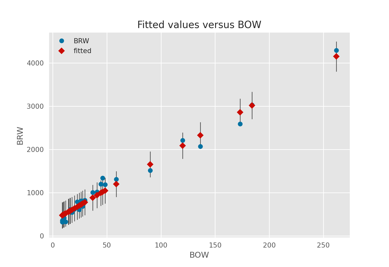

Tests sur les paramètres

On peut tester si une combinaison linéaire des paramètres est égale à 0:

combinaisons_lineaires = "Intercept = 0, BOW = 0, BOW - Intercept = 0, 3 * Intercept = 2 * BOW"
print(regression.t_test(combinaisons_lineaires))

##                              Test for Constraints                             
## ==============================================================================
##                  coef    std err          t      P>|t|      [0.025      0.975]
## ------------------------------------------------------------------------------
## c0           346.5452     35.492      9.764      0.000     273.590     419.500
## c1            14.5099      0.429     33.860      0.000      13.629      15.391
## c2          -332.0353     35.775     -9.281      0.000    -405.571    -258.500
## c3          1010.6157    107.040      9.441      0.000     790.592    1230.640
## ==============================================================================

Tests des effets

On peut tester les effets

from statsmodels.stats.anova import anova_lm
regression_multiple = smf.ols('BRW ~ BOW + AUD', data = batsphyto).fit()
anovaResults = anova_lm(regression_multiple, typ = "II") # On peut choisir le type
print(anovaResults)

##                 sum_sq    df           F        PR(>F)
## BOW       1.623042e+07   1.0  788.051516  2.007592e-20
## AUD       7.599175e+03   1.0    0.368970  5.490443e-01
## Residual  5.148909e+05  25.0         NaN           NaN

Tests de modèles emboités

anovaResults = anova_lm(regression, regression_multiple) # On peut choisir le type
print(anovaResults)

##    df_resid            ssr  df_diff      ss_diff        F    Pr(>F)
## 0      26.0  522490.111038      0.0          NaN      NaN       NaN
## 1      25.0  514890.935969      1.0  7599.175069  0.36897  0.549044

ANCOVA

Il semblerait que l’inclusion des variables qualitatives se déroule de la même manière que dans R. Exemple sur l’ANCOVA:

ancova = smf.ols('BRW ~ Clade * BOW', data = batsphyto).fit()
print(ancova.summary())

##                             OLS Regression Results                            
## ==============================================================================
## Dep. Variable:                    BRW   R-squared:                       0.979
## Model:                            OLS   Adj. R-squared:                  0.977
## Method:                 Least Squares   F-statistic:                     380.3
## Date:                Thu, 02 Sep 2021   Prob (F-statistic):           2.33e-20
## Time:                        10:48:17   Log-Likelihood:                -176.38
## No. Observations:                  28   AIC:                             360.8
## Df Residuals:                      24   BIC:                             366.1
## Df Model:                           3                                         
## Covariance Type:            nonrobust                                         
## ===================================================================================
##                       coef    std err          t      P>|t|      [0.025      0.975]
## -----------------------------------------------------------------------------------
## Intercept         379.6310     73.819      5.143      0.000     227.276     531.986
## Clade[T.II]       -21.6150     85.999     -0.251      0.804    -199.108     155.878
## BOW                14.5476      0.587     24.803      0.000      13.337      15.758
## Clade[T.II]:BOW    -0.8777      1.045     -0.840      0.409      -3.034       1.278
## ==============================================================================
## Omnibus:                        1.791   Durbin-Watson:                   1.808
## Prob(Omnibus):                  0.408   Jarque-Bera (JB):                0.733
## Skew:                           0.324   Prob(JB):                        0.693
## Kurtosis:                       3.457   Cond. No.                         350.
## ==============================================================================
## 
## Notes:
## [1] Standard Errors assume that the covariance matrix of the errors is correctly specified.

Moyennes ajustées

Il semblerait que, pour le moment, le calcul des moyennes ajustées doivent se faire à la main!

Graphes de diagnostics

On accède aux prédictions ou aux résidus avec les différents attributs de l’objet regression.

# model predictions
model_fitted_y = regression.fittedvalues
# model residuals
model_residuals = regression.resid

Il existe différents graphes de diagnostics qui diffèrent un peu de ceux de R

fig = plt.figure(figsize=(15,8))
sm.graphics.plot_regress_exog(regression, 'BOW', fig = fig)

plt.show()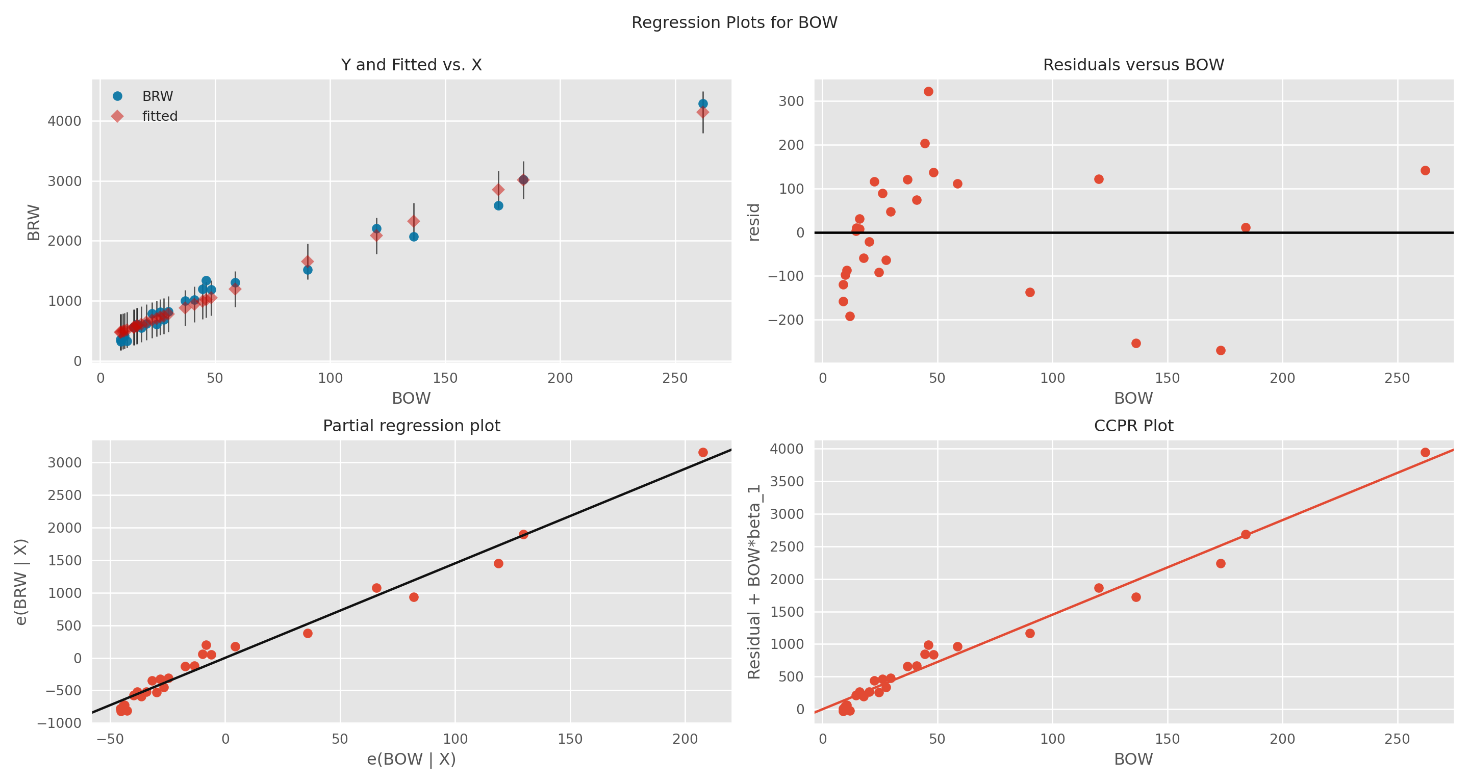

Graphique de l’influence

On peut obtenir le vecteur des distances de Cook grâce à la méthode get_influence

distances_cook = regression.get_influence().cooks_distance[0]

On peut tracer résidus standardisés en fonction du levier grâce à une fonction dédiée, graphique sans légende…

fig = sm.graphics.influence_plot(regression, criterion="cooks", alpha = 0.005)
plt.show()

## findfont: Font family ['sans-serif'] not found. Falling back to DejaVu Sans.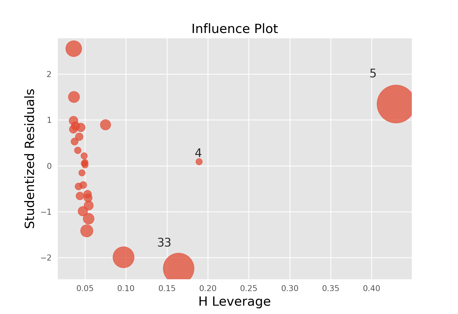

plt.figure(figsize=(6,5))

fig = sm.qqplot(regression.resid, stats.t, distargs=(4,), fit=True, line="45")
plt.show()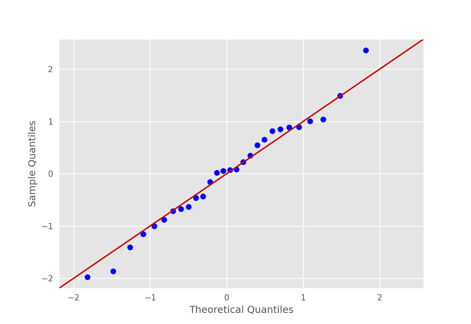

Quelques graphiques avec `seaborn`

Corrélations

# correlation heatmap 
bats3=bats[["BRW","BOW","AUD","MOB","HIP"]]
corr = bats3.corr()
plt.figure(figsize = (6,6))

sns.heatmap(corr, cmap="RdBu",
            xticklabels=corr.columns.values,
            yticklabels=corr.columns.values)

## <AxesSubplot:>

plt.show()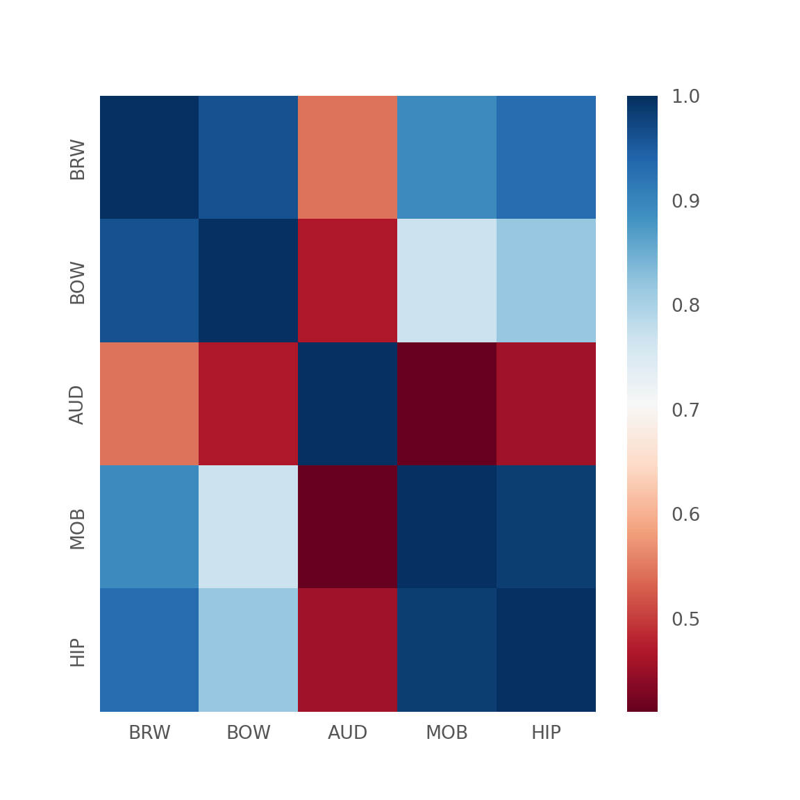

Boites à moustache

Attention, la variable groupe doit être en caractère impérativement.

sns.boxplot(x="BOW", y="Clade", data=bats,
            width=.6, palette="vlag")

# Add in points to show each observation

## <AxesSubplot:xlabel='BOW', ylabel='Clade'>

sns.stripplot(x="BOW", y="Clade", data=bats,
              size=4, color=".3", linewidth=0)

## <AxesSubplot:xlabel='BOW', ylabel='Clade'>

plt.show()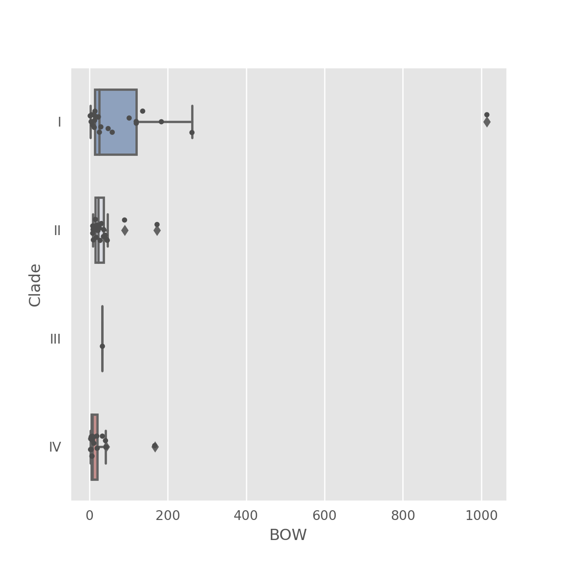

Pair plot

sns.set(style="ticks", color_codes=True)
sns.pairplot(bats3)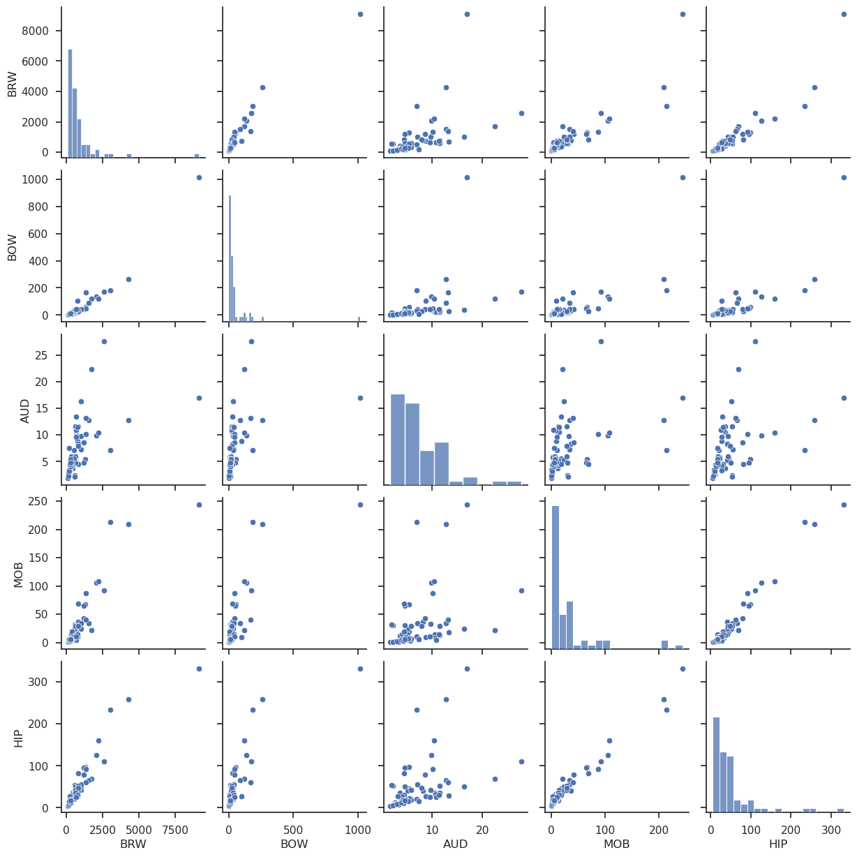

sns.pairplot(bats, hue="Clade")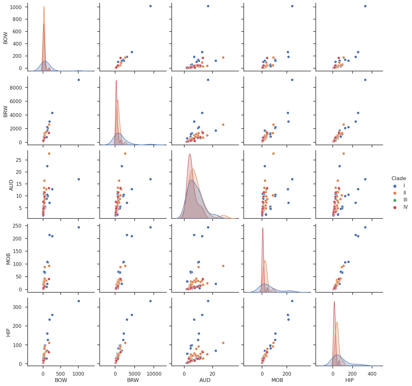

Regression plot

Attention les intervalles de confiance sont faits par bootstrap!

plt.figure(figsize = (5,5))

sns.regplot(x="BOW", y="BRW", data=bats);
plt.show()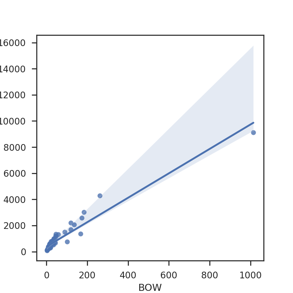

# le ; est indispensable pour que le graph s'affiche!
sns.lmplot(x="BOW", y="BRW", hue="Diet", data=bats);
plt.show()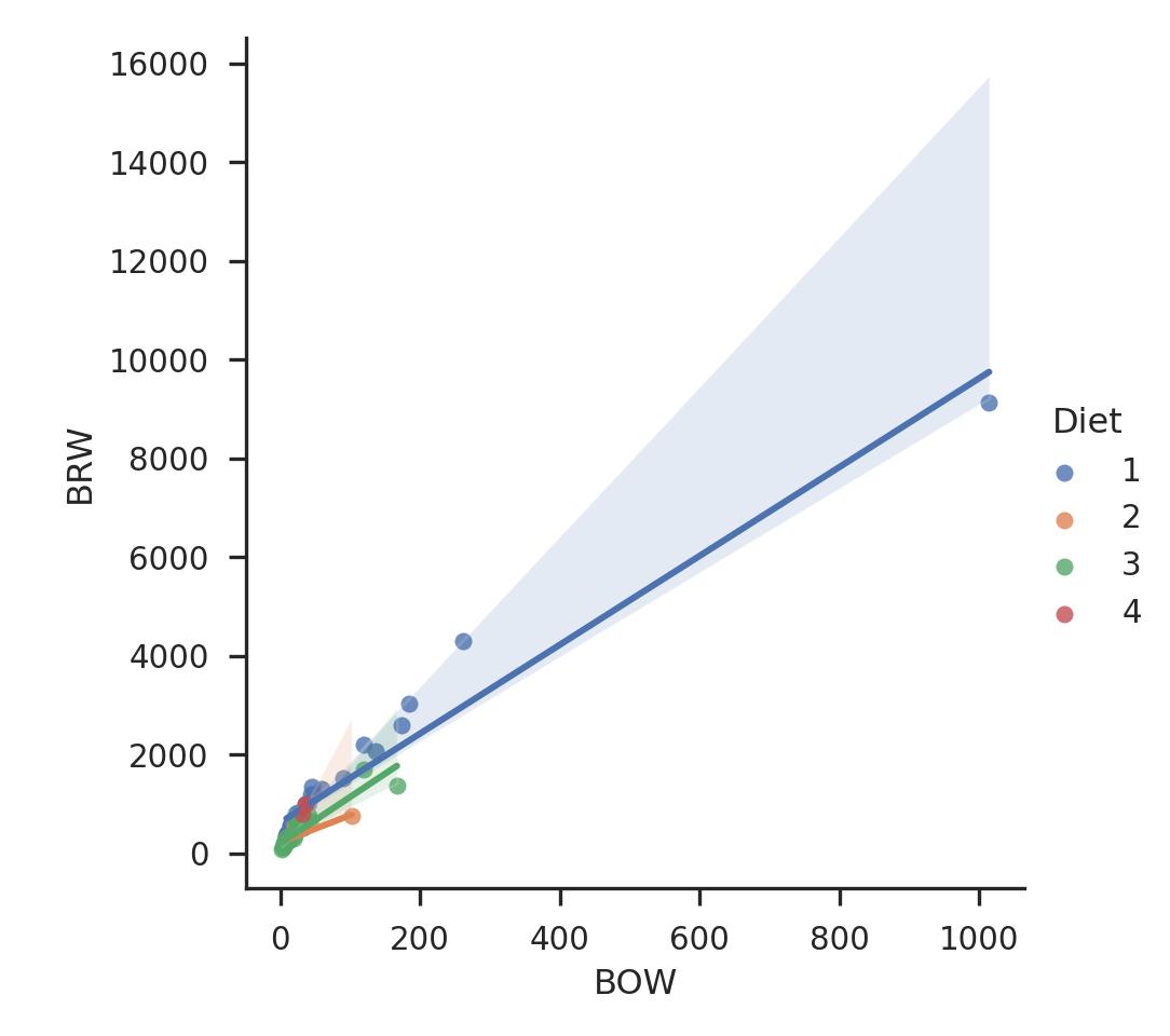

Complément sur les packages Python pour faire vos graphiques

bqplot : pour les graphes interactifs intégrés dans des notebooks.
seaborn : destinés aux statistiques et construit sur matplotlib.
toyplot : excellent pour tracer les graphes avec un très beau rendu pour le web.
bokeh : interactif qui fonctionne en mode serveur, c’est le Rshiny de Python.
pygal : si vous aimez les histogrammes et les camemberts.
Altair : pour tracer à partir d’une dataframe, construit sur la bibliothèque javascript vega. Magnifique rendu en html.
plot.ly : interactif et orienté sciences des données, fonctionne aussi avec R et Julia.
YT: orienté plus pour la physique mais excellent pour tracer des contours, des volumes, des surfaces et des particules.
Yellowbrick : compagnon graphique de scikit-learn.
scikit-plot : utile pour tracer les métriques issues de scikit-learn. Le développement semble à l’arrêt cependant.

lm en python

FinistR

26/08/2021

Objectif

Python depuis `rstudio`

Package `reticulate`

Installation des librairies python depuis `R`

Importation des modules python

Importation, manipulation et description des données

Import

Description

Changement de type d’une colonne

Première figure

Selection logique

Régression linéaire

Avec `scikit-learn`

Avec `statsmodels`

Tests sur les paramètres

Tests des effets

Tests de modèles emboités

ANCOVA

Moyennes ajustées

Graphes de diagnostics

Graphique de l’influence

Quelques graphiques avec `seaborn`

Corrélations

Boites à moustache

Pair plot

Regression plot

Complément sur les packages Python pour faire vos graphiques

lm en python

FinistR

26/08/2021

Objectif

Python depuis rstudio

Package reticulate

Installation des librairies python depuis R

Importation des modules python

Importation, manipulation et description des données

Import

Description

Changement de type d’une colonne

Première figure

Selection logique

Régression linéaire

Avec scikit-learn

Avec statsmodels

Tests sur les paramètres

Tests des effets

Tests de modèles emboités

ANCOVA

Moyennes ajustées

Graphes de diagnostics

Graphique de l’influence

Quelques graphiques avec seaborn

Corrélations

Boites à moustache

Pair plot

Regression plot

Complément sur les packages Python pour faire vos graphiques

Python depuis `rstudio`

Package `reticulate`

Installation des librairies python depuis `R`

Avec `scikit-learn`

Avec `statsmodels`

Quelques graphiques avec `seaborn`