Setting up simulations in R

Authors

Julie Aubert

Caroline Cognot

Annaïg De Walsche

Cédric Midoux

Pierre Neuvial

Aymeric Stamm

Florian Teste

Published

August 19, 2024

Overview

We explore several R packages for generate or structure simulations. Most statistical simulations studies includes different steps : generate data/ run one or several methods using simulated data / compare results.

We identified the following list of packages for data simulation:

{simulator}: A framework for performing simulations such as those common in methodological statistics papers. The design principles of this package are described in greater depth in Bien, J. (2016) “The simulator: An Engine to Streamline Simulations,” which is available at doi:10.48550/arXiv.1607.00021.
{simpr}: A general, ‘tidyverse’-friendly framework for simulation studies, design analysis, and power analysis. Specify data generation, define varying parameters, generate data, fit models, and tidy model results in a single pipeline, without needing loops or custom functions.
{DeclareDesign}: Researchers can characterize and learn about the properties of research designs before implementation using ‘DeclareDesign’. Ex ante declaration and diagnosis of designs can help researchers clarify the strengths and limitations of their designs and to improve their properties, and can help readers evaluate a research strategy prior to implementation and without access to results. It can also make it easier for designs to be shared, replicated, and critiqued.
{MonteCarlo}: Simplifies Monte Carlo simulation studies by automatically setting up loops to run over parameter grids and parallelising the Monte Carlo repetitions. It also generates LaTeX tables.
{simChef}: The goal is to help you quickly cook up a fully-realized, high-quality, reproducible, and transparently-documented simulation study in a flexible, efficient, and low-code manner. It removes many of the administrative burdens of simulation design through:
1. An intuitive tidy grammar of data science simulations
2. Powerful abstractions for distributed simulation processing backed by future
3. Automated generation of interactive R Markdown simulation documentation, situating results next to the workflows needed to reproduce them.
{simEngine}: An open-source R package for structuring, maintaining, running, and debugging statistical simulations on both local and cluster-based computing environments. See full documentation at https://avi-kenny.github.io/SimEngine/.

How to choose?

Here is a comparison of the different packages summarised in a table:

Name	Version	#deps	#rev deps	Latest commit	Latest release	On CRAN?	Developers
{DeclareDesign}	1.0.10	2	1	2024-04-13	2024-04-21	Yes	Graeme Blair
{MonteCarlo}	1.0.6	6	0	2019-01-31	2019-01-31	Yes	Christian Hendrik Leschinski
{simChef}	0.1.0	22	0	2024-03-20	NA	No	Tiffany Tang, James Duncan
{simEngine}	1.4.0	6	0	2024-04-13	2024-04-04	Yes	Avi Kenny, Charles Wolock
{simpr}	0.2.6	11	0	2024-07-16	2023-04-26	Yes	Ethan Brown
{simulator}	0.2.5	1	0	2023-02-02	2023-02-04	Yes	Jacob Bien

This table shows that all packages are on CRAN, except for {simChef}. The latest release of {simChef} is not available, but the latest commit was in March 2024 so it is actively maintained. The number of dependencies is quite high for {simChef} and {simpr}. The number of reverse dependencies is low for all packages. The package {MonteCarlo} seams not to be maintained anymore.

Also, in terms of philosophy, the {DeclareDesign} package is dedicated to experimental design. It also makes it possible to simulate an experimental design of interest, in order to understand the properties of this design. As its goal is not to evaluate computational methods via simulations, it does not address the question of interest and we did not evaluate it further. The underlying experimental design principles are described in the companion book: https://book.declaredesign.org/.

In the following, we will therefore focus on the packages {simEngine}, {simChef}, {simpr}, and {simulator}. The next section describes the common simulation problem we will use to compare the packages. Then, we will show how to solve this problem with each package. Finally, we will compare the packages based on the code, the output, and the ease of use.

A common simulation problem: power curve for test calibration

We consider a common simulation problem: power curve estimation for hypothesis test calibration.

We consider a two-sample paired t-test simple example. The first sample is generated from a normal distribution with mean 0 and standard deviation sd. The second sample is generated from a normal distribution with mean mean_diff and standard deviation sd. The sample size is n. We want to estimate the power of the paired t-test for different values of mean_diff and ds. Specifically, we will use the following parameters:

n: 100, 150, 200;
mean_diff: 10, 20, 30;
sd: 50, 100.

We will estimate the power by simulating the paired t-test for each combination of parameters. We will repeat the simulation 10 times for each combination of parameters.

The base R solution for this problem can look like this:

## Set up parameters
ns <- c(100L, 150L, 200L)
mean_diffs <- c(10, 20, 30)
sds <- c(50, 100)
reps <- 10L

## Bring together into data frame
results_template <- expand.grid(
  n = ns, 
  mean_diff = mean_diffs, 
  sd = sds, 
  p.value = NA_real_
)
base_r_sim <- results_template[rep(1:nrow(results_template), each = reps), ]

## Loop over rows of the data frame and calculate the p-value
for (i in 1:nrow(results_template)) {
  params <- base_r_sim[i,]
  pre <- rnorm(params$n, 0, params$sd)
  post <- pre + rnorm(params$n, params$mean_diff, params$sd)
  base_r_sim$p.value[i] <- t.test(pre, post)$p.value
}

## Display table output
DT::datatable(base_r_sim)

{simpr}

What is bad in the base R solution according to {simpr} authors:

Most important pieces (data generating process, model specification, definitions, varying parameters) are hidden;
What if there is an error?
What about parallelization?
Is this code sufficiently readable? Without the comments?

{simpr} solution

simpr_tbl <- specify(
  pre  = ~ rnorm(n, 0, sd),
  post = ~ pre + rnorm(n, mean_diff, sd)
) |> 
  define(n = ns, mean_diff = mean_diffs, sd = sds) |> 
  generate(reps, .progress = TRUE) |> 
  fit(t = ~ t.test(post, pre, paired = TRUE)) |> 
  tidy_fits()


Attaching package: 'purrr'

The following object is masked from 'package:magrittr':

    set_names

DT::datatable(simpr_tbl)

simpr_tbl |> 
  dplyr::group_by(n, mean_diff, sd) |> 
  dplyr::summarize(Power = mean(p.value < 0.05)) |> 
  dplyr::ungroup() |> 
  ggplot(aes(n, Power)) + 
  geom_col() + 
  facet_grid(rows = dplyr::vars(sd), cols = dplyr::vars(mean_diff)) + 
  theme_bw()

`summarise()` has grouped output by 'n', 'mean_diff'. You can override using
the `.groups` argument.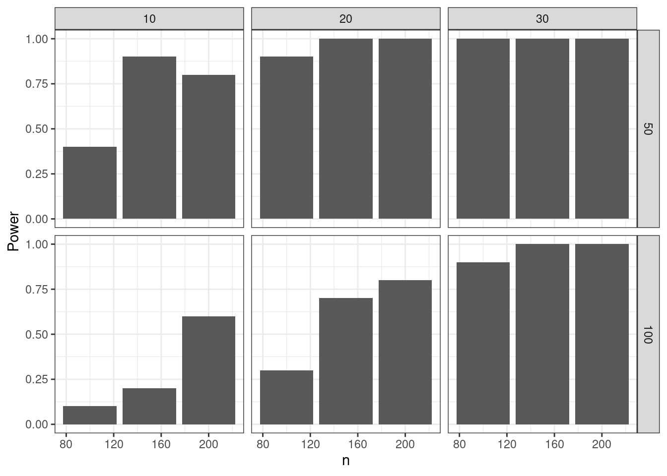

Philosophy

The {simpr} workflow, inspired by the {infer} package, distills a simulation study into five primary steps:

specify() your data-generating process;
define() parameters that you want to systematically vary across your simulation design (e.g. n, effect size);
generate() the simulation data;
fit() models to your data (e.g. lm());
tidy_fits() for consolidating results using broom::tidy(), such as computing power or Type I Error rates.

Reproducible workflows

Same seed, same results;
Can regenerate just a specific subset to see what happened in that particular dataset or fit;
Useful in debugging and diagnosing unexpected results, etc.

Filtering full simulation

withr::with_seed(500, {
  specify(a = ~ runif(6)) |> 
    generate(3) |> 
    dplyr::filter(.sim_id == 3)
})

full tibble
--------------------------
# A tibble: 1 × 3
  .sim_id   rep sim             
    <int> <int> <list>          
1       3     3 <tibble [6 × 1]>

sim[[1]]
--------------------------
# A tibble: 6 × 1
      a
  <dbl>
1 0.371
2 0.959
3 0.633
4 0.177
5 0.803
6 0.133

Simulate subset only

withr::with_seed(500, {
  specify(a = ~ runif(6)) |> 
    generate(3, .sim_id == 3)
})

full tibble
--------------------------
# A tibble: 1 × 3
  .sim_id   rep sim             
    <int> <int> <list>          
1       3     3 <tibble [6 × 1]>

sim[[1]]
--------------------------
# A tibble: 6 × 1
      a
  <dbl>
1 0.371
2 0.959
3 0.633
4 0.177
5 0.803
6 0.133

Benchmarking

bench::mark(
  all = specify(a = ~ runif(6)) |> 
    generate(1000) |> 
    dplyr::filter(.sim_id == 1000),
  subset = specify(a = ~ runif(6)) |> 
    generate(1000, .sim_id == 1000),
  check = FALSE, min_iterations = 10L, relative = TRUE
)

Warning: Some expressions had a GC in every iteration; so filtering is
disabled.

# A tibble: 2 × 6
  expression   min median `itr/sec` mem_alloc `gc/sec`
  <bch:expr> <dbl>  <dbl>     <dbl>     <dbl>    <dbl>
1 all         65.5   63.3       1        1        1   
2 subset       1      1        64.1      1.29     1.26

Other features

Data munging

Add per_sim() |> after generate() in your simulation pipeline and then any tidyverse function that will apply to every simulation dataset:

specify(
  pre  = ~ rnorm(n, 0, sd), 
  post = ~ pre + rnorm(n, mean_diff, sd)
) |> 
  define(n = ns, mean_diff = mean_diffs, sd = sds) |> 
  generate(reps, .progress = TRUE) |> 
  ## Apply tidyverse functions to every simulation dataset
  per_sim() |> 
  ## Mutate to add a range restriction
  dplyr::mutate(dplyr::across(dplyr::everything(), dplyr::case_when(
    pre >  100 ~ 100,
    pre < -100 ~ -100,
    .default   ~ pre
  ))) |> 
  fit(t = ~ t.test(post, pre, paired = TRUE)) |> 
  tidy_fits()

Error handling

Can change error handling to keep going with simulation, stop simulation, or to skip warnings;
Debug and recovery options to enter into simulation during error.

Built-in parallelization

Just add

library(future)
plan(multisession, workers = 6) # or however many cores are reasonable to use

and your simulation pipeline (actually the generate() function) will run in parallel.

Pros & cons

Pros

tidyverse friendly;
beginner friendly;
Reproducibility, error handling built in;
General-purpose, customizable and can handle arbitrary R code.

Cons

Likely not as fast/optimized as some alternatives;
Not as customizable/powerful as DeclareDesign;
Not specifically set up for any particular application (no MC errors, plots, reports, specific models…).

{simulator}

This is a package on the CRAN. It is described in a 2016 paper by Jacob Bien. Last update on GitHub : last year (so, 2023).

Getting started

The function create(), with a directory that does not exist, will create the directory with 5 files and 1 folder:

eval_functions.R: contains metrics to be evaluated;
files/: directory to store results;
main.R: main code to run;
method_functions.R: methods to run;
model_functions.R: define the models;
writeup.Rmd.

simulator_dir <- "./sims_simulator"
if (!file.exists(simulator_dir))
  create(simulator_dir)

New simulation template created!  Go to ./sims_simulator/main.R to get started.

withr::with_dir(simulator_dir, {
  list.files()
})

[1] "eval_functions.R"   "main.R"             "method_functions.R"
[4] "model_functions.R"  "writeup.Rmd"

On a typical project, one starts by defining a model in model_functions.R, one or two methods in method_functions.R, and a few metrics in eval_functions.R, and then one runs the code in main.R. After looking at some of the results, one might add an additional model or method or metric. One then returns to main.R, adds some additional lines specifying that the additional components should be run as well and looks at some more results.

The simplest way to look at results is by using the plot functions plot_eval(), plot_evals() and plot_evals_by(). In situations where you wish to investigate results more deeply than just looking at aggregated plots, one can use the functions model(), draws(), output(), and evals() to get at all objects generated through the course of the simulation.

The create() function also creates the template in the different files:

Content of `model_functions.R`

make_my_model <- function(n, prob) {
  new_model(
    name = "contaminated-normal", 
    label = sprintf("Contaminated normal (n = %s, prob = %s)", n, prob), 
    params = list(n = n, mu = 2, prob = prob), 
    simulate = function(n, mu, prob, nsim) {
      # this function must return a list of length nsim
      contam <- runif(n * nsim) < prob
      x <- matrix(rep(NA, n * nsim), n, nsim)
      x[contam] <- rexp(sum(contam))
      x[!contam] <- rnorm(sum(!contam))
      x <- mu + x # true mean is mu
      return(split(x, col(x))) # make each col its own list element
    }
  )
}

Define a model from its different components with new_model():

name;
label: what will be printed in the tables later probably?
param: a list of different parameters for the model;
simulate: a function of the parameters that returns nsim simulations.

Content of `method_functions.R`

my_method <- new_method(
  name = "my-method", 
  label = "My Method", 
  method = function(model, draw) {
    list(fit = median(draw))
  }
)

their_method <- new_method(
  name = "their-method", 
  label = "Their Method",
  method = function(model, draw) {
    list(fit = mean(draw))
  }
)

Define methods to be used on the model. The function new_method() has for arguments a name (for R) name, a pretty name label, and the method named arg for the computation we want.

Content of `eval_functions.R`

his_loss <- new_metric(
  name = "hisloss", 
  label = "His loss function",
  metric = function(model, out) {
    return((model$mu - out$fit)^2)
  }
)

her_loss <- new_metric(
  name = "herloss", 
  label = "Her loss function",
  metric = function(model, out) {
    return(abs(model$mu - out$fit))
  }
)

Metric objects: shows how to compare model object and output of the method (method used on sim) object.

Content of `main.R`

setwd(simulator_dir)

source("model_functions.R")
source("method_functions.R")
source("eval_functions.R")

## @knitr init

name_of_simulation <- "normal-mean-estimation-with-contamination"

## @knitr main

sim <- new_simulation(
  name = name_of_simulation,
  label = "Mean estimation under contaminated normal"
) %>%
  generate_model(
    make_model = make_my_model, 
    seed = 123,
    n = 50,
    prob = as.list(seq(0, 1, length = 6)),
    vary_along = "prob"
  ) %>%
  simulate_from_model(nsim = 10) %>%
  run_method(list(my_method, their_method)) %>%
  evaluate(list(his_loss, her_loss))

## @knitr plots

plot_eval_by(sim = sim, metric_name = "hisloss", varying = "prob")

## @knitr tables

tabulate_eval(
  object = sim, 
  metric_name = "herloss", 
  output_type = "markdown",
  format_args = list(digits = 1)
)

The main.R script calls the different files.

Can plot_eval_by() be used for different metrics at once? Can tabulate_eval() be used for different metrics at once?

Example: power curve

Here is the content of the main.R file in the folder simulator_equality_test/.

library(simulator) # this file was created under simulator version 0.2.5

source("simulator_equality_test/model_functions.R")
source("simulator_equality_test/method_functions.R")
source("simulator_equality_test/eval_functions.R")

## @knitr init

name_of_simulation <- "normal-mean-test"

## @knitr main

f <- file()
sink(file = f)

sim <- new_simulation(
  name = name_of_simulation, 
  label = "Test of mean"
) |> 
  generate_model(
    make_model = make_my_model_normal, 
    seed = 13, 
    n = 20, 
    mu2 = as.list(seq(0, 10, by = 0.5)), 
    mu1 = 0, 
    sig = 5, 
    vary_along = "mu2"
  ) |> 
  simulate_from_model(nsim = 1000) |> 
  run_method(list(t_test)) |> 
  evaluate(list(pval_loss))

..Created model and saved in normal/mu1_0/mu2_0/n_20/sig_5/model.Rdata
..Created model and saved in normal/mu1_0/mu2_0.5/n_20/sig_5/model.Rdata
..Created model and saved in normal/mu1_0/mu2_1/n_20/sig_5/model.Rdata
..Created model and saved in normal/mu1_0/mu2_1.5/n_20/sig_5/model.Rdata
..Created model and saved in normal/mu1_0/mu2_2/n_20/sig_5/model.Rdata
..Created model and saved in normal/mu1_0/mu2_2.5/n_20/sig_5/model.Rdata
..Created model and saved in normal/mu1_0/mu2_3/n_20/sig_5/model.Rdata
..Created model and saved in normal/mu1_0/mu2_3.5/n_20/sig_5/model.Rdata
..Created model and saved in normal/mu1_0/mu2_4/n_20/sig_5/model.Rdata
..Created model and saved in normal/mu1_0/mu2_4.5/n_20/sig_5/model.Rdata
..Created model and saved in normal/mu1_0/mu2_5/n_20/sig_5/model.Rdata
..Created model and saved in normal/mu1_0/mu2_5.5/n_20/sig_5/model.Rdata
..Created model and saved in normal/mu1_0/mu2_6/n_20/sig_5/model.Rdata
..Created model and saved in normal/mu1_0/mu2_6.5/n_20/sig_5/model.Rdata
..Created model and saved in normal/mu1_0/mu2_7/n_20/sig_5/model.Rdata
..Created model and saved in normal/mu1_0/mu2_7.5/n_20/sig_5/model.Rdata
..Created model and saved in normal/mu1_0/mu2_8/n_20/sig_5/model.Rdata
..Created model and saved in normal/mu1_0/mu2_8.5/n_20/sig_5/model.Rdata
..Created model and saved in normal/mu1_0/mu2_9/n_20/sig_5/model.Rdata
..Created model and saved in normal/mu1_0/mu2_9.5/n_20/sig_5/model.Rdata
..Created model and saved in normal/mu1_0/mu2_10/n_20/sig_5/model.Rdata
..Simulated 1000 draws in 0.01 sec and saved in normal/mu1_0/mu2_0/n_20/sig_5/r1.Rdata
..Simulated 1000 draws in 0.01 sec and saved in normal/mu1_0/mu2_0.5/n_20/sig_5/r1.Rdata
..Simulated 1000 draws in 0.01 sec and saved in normal/mu1_0/mu2_1/n_20/sig_5/r1.Rdata
..Simulated 1000 draws in 0.01 sec and saved in normal/mu1_0/mu2_1.5/n_20/sig_5/r1.Rdata
..Simulated 1000 draws in 0.01 sec and saved in normal/mu1_0/mu2_2/n_20/sig_5/r1.Rdata
..Simulated 1000 draws in 0.01 sec and saved in normal/mu1_0/mu2_2.5/n_20/sig_5/r1.Rdata
..Simulated 1000 draws in 0.01 sec and saved in normal/mu1_0/mu2_3/n_20/sig_5/r1.Rdata
..Simulated 1000 draws in 0 sec and saved in normal/mu1_0/mu2_3.5/n_20/sig_5/r1.Rdata
..Simulated 1000 draws in 0.01 sec and saved in normal/mu1_0/mu2_4/n_20/sig_5/r1.Rdata
..Simulated 1000 draws in 0 sec and saved in normal/mu1_0/mu2_4.5/n_20/sig_5/r1.Rdata
..Simulated 1000 draws in 0.01 sec and saved in normal/mu1_0/mu2_5/n_20/sig_5/r1.Rdata
..Simulated 1000 draws in 0.01 sec and saved in normal/mu1_0/mu2_5.5/n_20/sig_5/r1.Rdata
..Simulated 1000 draws in 0.01 sec and saved in normal/mu1_0/mu2_6/n_20/sig_5/r1.Rdata
..Simulated 1000 draws in 0.01 sec and saved in normal/mu1_0/mu2_6.5/n_20/sig_5/r1.Rdata
..Simulated 1000 draws in 0 sec and saved in normal/mu1_0/mu2_7/n_20/sig_5/r1.Rdata
..Simulated 1000 draws in 0.01 sec and saved in normal/mu1_0/mu2_7.5/n_20/sig_5/r1.Rdata
..Simulated 1000 draws in 0.01 sec and saved in normal/mu1_0/mu2_8/n_20/sig_5/r1.Rdata
..Simulated 1000 draws in 0.01 sec and saved in normal/mu1_0/mu2_8.5/n_20/sig_5/r1.Rdata
..Simulated 1000 draws in 0.01 sec and saved in normal/mu1_0/mu2_9/n_20/sig_5/r1.Rdata
..Simulated 1000 draws in 0.01 sec and saved in normal/mu1_0/mu2_9.5/n_20/sig_5/r1.Rdata
..Simulated 1000 draws in 0.01 sec and saved in normal/mu1_0/mu2_10/n_20/sig_5/r1.Rdata
..Performed Mean equality test in 0 seconds (on average over 1000 sims)
..Performed Mean equality test in 0 seconds (on average over 1000 sims)
..Performed Mean equality test in 0 seconds (on average over 1000 sims)
..Performed Mean equality test in 0 seconds (on average over 1000 sims)
..Performed Mean equality test in 0 seconds (on average over 1000 sims)
..Performed Mean equality test in 0 seconds (on average over 1000 sims)
..Performed Mean equality test in 0 seconds (on average over 1000 sims)
..Performed Mean equality test in 0 seconds (on average over 1000 sims)
..Performed Mean equality test in 0 seconds (on average over 1000 sims)
..Performed Mean equality test in 0 seconds (on average over 1000 sims)
..Performed Mean equality test in 0 seconds (on average over 1000 sims)
..Performed Mean equality test in 0 seconds (on average over 1000 sims)
..Performed Mean equality test in 0 seconds (on average over 1000 sims)
..Performed Mean equality test in 0 seconds (on average over 1000 sims)
..Performed Mean equality test in 0 seconds (on average over 1000 sims)
..Performed Mean equality test in 0 seconds (on average over 1000 sims)
..Performed Mean equality test in 0 seconds (on average over 1000 sims)
..Performed Mean equality test in 0 seconds (on average over 1000 sims)
..Performed Mean equality test in 0 seconds (on average over 1000 sims)
..Performed Mean equality test in 0 seconds (on average over 1000 sims)
..Performed Mean equality test in 0 seconds (on average over 1000 sims)
..Evaluated Mean equality test in terms of pval<0.05, Computing time (sec)
..Evaluated Mean equality test in terms of pval<0.05, Computing time (sec)
..Evaluated Mean equality test in terms of pval<0.05, Computing time (sec)
..Evaluated Mean equality test in terms of pval<0.05, Computing time (sec)
..Evaluated Mean equality test in terms of pval<0.05, Computing time (sec)
..Evaluated Mean equality test in terms of pval<0.05, Computing time (sec)
..Evaluated Mean equality test in terms of pval<0.05, Computing time (sec)
..Evaluated Mean equality test in terms of pval<0.05, Computing time (sec)
..Evaluated Mean equality test in terms of pval<0.05, Computing time (sec)
..Evaluated Mean equality test in terms of pval<0.05, Computing time (sec)
..Evaluated Mean equality test in terms of pval<0.05, Computing time (sec)
..Evaluated Mean equality test in terms of pval<0.05, Computing time (sec)
..Evaluated Mean equality test in terms of pval<0.05, Computing time (sec)
..Evaluated Mean equality test in terms of pval<0.05, Computing time (sec)
..Evaluated Mean equality test in terms of pval<0.05, Computing time (sec)
..Evaluated Mean equality test in terms of pval<0.05, Computing time (sec)
..Evaluated Mean equality test in terms of pval<0.05, Computing time (sec)
..Evaluated Mean equality test in terms of pval<0.05, Computing time (sec)
..Evaluated Mean equality test in terms of pval<0.05, Computing time (sec)
..Evaluated Mean equality test in terms of pval<0.05, Computing time (sec)
..Evaluated Mean equality test in terms of pval<0.05, Computing time (sec)

sink()
close(f)
unlink(f)

## @knitr tables

tabulate_eval(
  sim, 
  metric_name = "p_value", 
  output_type = "markdown",
  format_args = list(digits = 5)
)

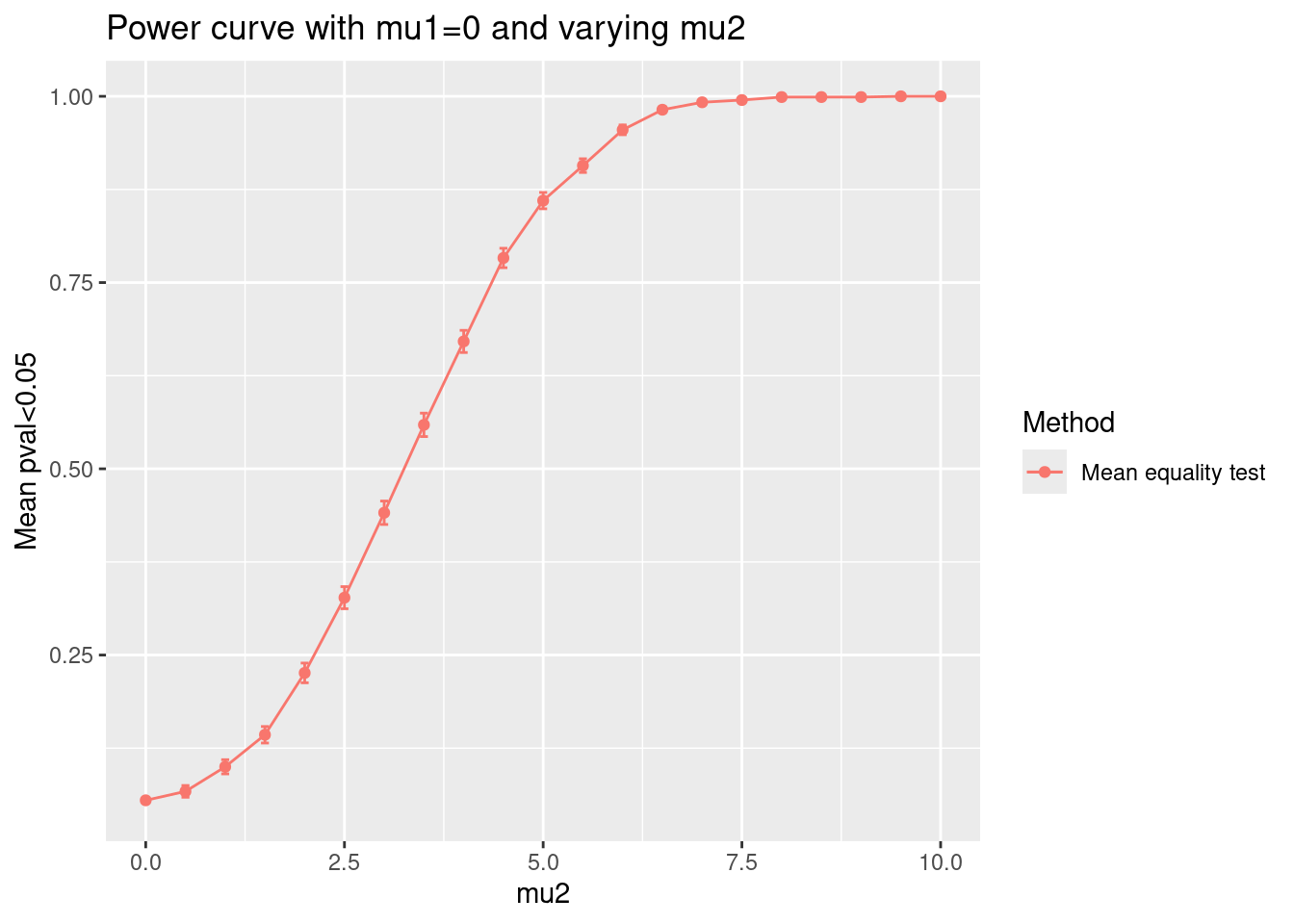
<!-- generated by simulator on Thu Sep 12 08:15:13 2024. -->

A comparison of Mean pval<0.05 (averaged over 1000 replicates).
	Mean equality test
normal	0.055 (0.0072130)
normal	0.067 (0.0079103)
normal	0.100 (0.0094916)
normal	0.143 (0.0110758)
normal	0.226 (0.0132325)
normal	0.327 (0.0148422)
normal	0.441 (0.0157088)
normal	0.559 (0.0157088)
normal	0.671 (0.0148654)
normal	0.783 (0.0130415)
normal	0.860 (0.0109782)
normal	0.907 (0.0091889)
normal	0.955 (0.0065588)
normal	0.982 (0.0042064)
normal	0.992 (0.0028185)
normal	0.995 (0.0022316)
normal	0.999 (0.0010000)
normal	0.999 (0.0010000)
normal	0.999 (0.0010000)
normal	1.000 (0.0000000)
normal	1.000 (0.0000000)

## @knitr plots

plot_eval_by(
  sim, 
  metric_name = "p_value", 
  varying = "mu2", 
  main = "Power curve with mu1=0 and varying mu2"
)

ToDo :

vary n
vary both n and mu2

Important functions

new_model();
new_method();
new_metric();
new_simulation();
generate_model();
simulate_from_model();
run_method();
evaluate();
plot_eval(), plot_eval_by(), tabulate_eval().

Pros & cons

This is not really a package that codes a method, but instead it proposes an architecture to store your codes, output simulations, results, etc.

Pros

any model possible, if you can write it;
possible to iterate over parameter with pretty pipes;
parallel possible, because you choose what you use;
stores all results in the storage with increasing depth:

files
└── name_of_model
    └── name_of_first_param_value
        └── name_of2nd_param_value ... model.Rdata out stores all sims
            └── r?.Rdata

Cons

Not an usual way to code in R, and not easy to explain. Create the directory with the create() function. Then, add the different functions, methods, models, etc., in the corresponding files;
Mixes the code of the package/template with your own code;
Stores all results in this neat way BUT if too many parameters, may exceed the depth allowed.

{simEngine}

{simEngine} is an open-source R package for structuring, maintaining, running, and debugging statistical simulations on both local and cluster-based computing environments. The paper describing the package is available here.

Example

Create a simulation object SimEngine::new_sim()

sim <- new_sim()

Create functions to generate data

create_data <- function(n) {
  return(rpois(n = n, lambda = 20))
}

est_lambda <- function(dat, type) {
  if (type=="M") {
    return(mean(dat))
  }
  if (type=="V") {
    return(var(dat))
  }
}

Simulation set-up

One run = one simulation replicate. Features varying across simulation = simulation levels. Possible values = level values. By default, {simEngine} runs one simulation replicate for each combination of level value.

sim <- sim |> 
  set_levels(
    estimator = c("M", "V"),
    n = c(10, 100, 1000)
  )
sim

SimEngine: simulation object (class "sim_obj")
----------------------------------------------
Configuration: 
    num_sim: 1
    parallel: FALSE
    n_cores: NA
    packages: NULL
    stop_at_error: FALSE
    seed: 528361534
    progress_bar: TRUE
    batch_levels: NA
    return_batch_id: FALSE
Levels: 
    estimator: c("M", "V")
    n: c(10, 100, 1000)
State: pre run

Create a simulation script

i.e. generation, analysis and return results

sim <- sim |> 
  set_script(function() {
    dat <- create_data(n = L$n)
    lambda_hat <- est_lambda(dat = dat, type = L$estimator)
    return(list("lambda_hat" = lambda_hat))
  })

Configure and run the simulation

Using the SimEngine::set_config() it is possible to specify the number of replicates num_sim, the parallelization type n_cores, parallel, … and the required packages packages argument.

And we run the simulation with the SimEngine::run() function.

### Configuration
sim <- sim |> 
  set_config(
    num_sim = 100,
    packages = c("ggplot2", "stringr")
  )

### Run
sim <- run(sim)

Done. No errors or warnings detected.

The package implements a SimEngine::summarize() function to calculate usual summary statistics such as bias, variance, MSE.

sim |> 
  summarize(
    list(
      stat = "bias",
      name = "bias_lambda",
      estimate = "lambda_hat",
      truth = 20
    ), 
    list(
      stat = "mse",
      name = "mse_lambda",
      estimate = "lambda_hat",
      truth = 20
    )
  )

  level_id estimator    n n_reps bias_lambda  mse_lambda
1        1         M   10    100  -0.0930000  1.75850000
2        2         V   10    100   0.3353333 96.23611111
3        3         M  100    100  -0.0877000  0.20287100
4        4         V  100    100  -0.3656687  9.04930168
5        5         M 1000    100   0.0198000  0.02163858
6        6         V 1000    100   0.1130303  0.75417061

We can have information on individual simulation including runtime.

head(sim$results)

  sim_uid level_id rep_id estimator  n      runtime lambda_hat
1       1        1      1         M 10 0.0007116795       20.3
2       7        1      2         M 10 0.0005488396       20.4
3       8        1      3         M 10 0.0005645752       19.8
4       9        1      4         M 10 0.0005791187       19.1
5      10        1      5         M 10 0.0005605221       19.8
6      11        1      6         M 10 0.0005788803       20.9

It is possible to update simulation with more replicates or a new level. It keeps the old simulations and run only needed ones.

sim <- sim |> 
  set_config(num_sim = 200) |> 
  set_levels(
    estimator = c("M", "V"),
    n = c(10, 100, 1000, 10000)
  ) |> 
  update_sim()

Done. No errors or warnings detected.

Parallelization

A specific vignette is available and the introduction precises the terminology for parallel computing (node, core, task, job, etc.). There are two modes of parallelizing code: local or cluster. The first thing is to specify set_config(parallel = TRUE).

Local: split calculations on several cores of a single computer. If the user’s computer has \(n\) cores available, {simEngine} will use \(n-1\) cores by default.
Cluster: function run_on_cluster(). To use the function, the user needs to break the code into three blocks : first (code run only once, set-up simulation object), main (a single call to run()) and last (the code will run after all simulation replicates have finished running and after SimEngine has automatically compiled the results into the simulation object.).

run_on_cluster(
  first = {
    create_data <- function(n) {
      return(rpois(n = n, lambda = 20))
    }
    est_lambda <- function(dat, type) {
      if (type == "M") {
        return(mean(dat))
      }
      if (type == "V") {
        return(var(dat))
      }
    }
    sim <- new_sim() |> 
      set_levels(estimator = c("M", "V"), n = c(10, 100, 1000)) |> 
      set_script(function() {
        dat <- create_data(L$n)
        lambda_hat <- est_lambda(dat = dat, type = L$estimator)
        return(list("lambda_hat" = lambda_hat))
      }) |> 
      set_config(num_sim = 100, n_cores = 20)
  },
  main = {
    sim <- run(sim)
  },
  last = {
    sim <- summarize(sim)
  },
  cluster_config = list(js = "slurm")
)

Done. No errors or warnings detected.

The cluster_config argument enables to specify options such as the choice of the scheduler.

Example on how to give instruction to the job scheduler is on the vignette.

Be caution: the number of cores cannot exceed the total number of simulation replicates.

Function to update simulation on a CSS: update_sim_on_cluster(). Difference is we do not need to create a new simulation config but load the existing simulation using readRDS() and use set_config() or set_levels() and update_sim() in the main block.

There is a vignette on advanced functionality such as complex results or simulation levels. It exists the batch() function to share data or objects between simulation replicates.

Pros & cons

Pros

beginner friendly;
local and cluster-based computing environments;
well-written documentations and website with vignettes (with stat. formula of terminology for parallel computing);
information-sharing across simulation replicates (not tested);
automatic calculation of Monte Carlo error (not tested).

Cons

Simulation-based power calculation

A [specific vignette] is available on the author’s website.

{simChef}

This document describes a simulation experiment using the {simChef} package in R, including data generation, method application, evaluation, and visualization.

A specific vignette is available on the author’s website for more detailed instructions and examples on using the {simChef} package.

Setup

The {simChef} package is not on CRAN and must therefore be installed from GitHub using the {remotes} package as follows:

remotes::install_github("Yu-Group/simChef")

In {simChef}, a simulation experiment is divided into four components:

DGP(): the data-generating processes (DGPs) from which to generate data;
Method(): the methods (or models) to fit on the data in the experiment;
Evaluator(): the evaluation metrics used to evaluate the methods’ performance;
Visualizer(): the visualization procedures used to visualize outputs from the method fits or evaluation results (can be tables, plots, or even R Markdown snippets to display).

Step 1: Define the Data-Generating Process, Methods, and Evaluation Functions

Data-Generating Process

The following function generates pre- and post-treatment data:

dgp_fun <- function(n, sd, mean_diff) {
  pre  <- rnorm(n, 0, sd)
  post <- pre + rnorm(n, mean_diff, sd)
  list(pre = pre, post = post)
}

Method

The following function applies a paired t-test to the data:

method_fun <- function(pre, post) {
  t.test(post, pre, paired = TRUE)
}

Evaluation

The following function evaluates the power of the test:

evaluation_fun <- function(fit_results) {
  Power <- fit_results |> 
    dplyr::group_by(n, mean_diff, sd) |> 
    dplyr::summarize(Power = mean(p.value < 0.05))
}

Visualization

The following function creates a plot to visualize the power:

power_plot_fun <- function(fit_results, eval_results) {
  fit_results |> 
    dplyr::group_by(n, mean_diff, sd) |> 
    dplyr::summarize(Power = mean(p.value < 0.05)) |> 
    ggplot(aes(n, Power)) + 
    geom_col() + 
    facet_grid(rows = dplyr::vars(sd), cols = dplyr::vars(mean_diff)) + 
    theme_bw()
}

Step 2: Convert Functions into {simChef} Class Objects

dgp <- create_dgp(
  .dgp_fun = dgp_fun, .name = "DGP"
)

method <- create_method(
  .method_fun = method_fun, .name = "T-test"
)

evaluation <- create_evaluator(
  .eval_fun = evaluation_fun , .name = 'P.value'
)

power_plot <- create_visualizer(
  .viz_fun = power_plot_fun, .name = 'Power plot'
)

Step 3: Assemble the Simulation Experiment

experiment <- create_experiment(name = "Example Experiment") |> 
  add_dgp(dgp) |> 
  add_method(method) |> 
  add_evaluator(evaluation) |> 
  add_visualizer(power_plot)

## Define the grid of simulation parameters
experiment <- experiment |> 
  add_vary_across(.dgp = "DGP", n = ns, mean_diff = mean_diffs, sd = sds)

print(experiment)

Experiment Name: Example Experiment 
   Saved results at: results/Example Experiment 
   DGPs: DGP 
   Methods: T-test 
   Evaluators: P.value 
   Visualizers: Power plot 
   Vary Across: 
      DGP: DGP 
         n:  int [1:3] 100 150 200
         mean_diff:  num [1:3] 10 20 30
         sd:  num [1:2] 50 100

Step 4: Run the Experiment

results <- run_experiment(experiment, n_reps = reps, save = TRUE)

Fitting Example Experiment...
Saving fit results...
Fit results saved | time taken: 0.015704 seconds
10 reps completed (totals: 10/10) | time taken: 0.680623 minutes
==============================
Evaluating Example Experiment...
`summarise()` has grouped output by 'n', 'mean_diff'. You can override using the `.groups` argument.
Evaluation completed | time taken: 0.000174 minutes
Saving eval results...
Eval results saved | time taken: 0.051551 seconds
==============================
Visualizing Example Experiment...
`summarise()` has grouped output by 'n', 'mean_diff'. You can override using the `.groups` argument.
Visualization completed | time taken: 0.000305 minutes
Saving viz results...
Viz results saved | time taken: 0.072612 seconds
==============================

DT::datatable(results$fit_results)

results$viz_results

$`Power plot`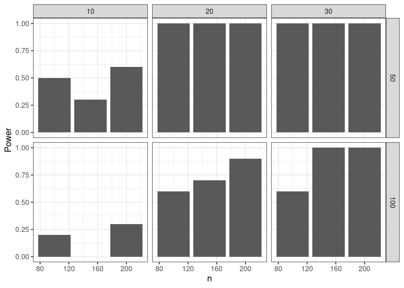

Pros & cons

Pros

Automated generation of an interactive R Markdown document (see init_docs() and render_docs() functions);
Beginner friendly;
Computing experimental replicates in parallel easily with future by adding plan(multisession, workers = n_workers) before run_experiment(experiment, ...);
Flexibility of the return fitting results of the simulation (not necessarily the same outputs for all methods);
We can change the evaluation metrics and the visualization without re-fitting all the simulations by saving the fit_results tibble.

Cons

Likely not as fast/optimized as some alternatives;
Only save the simulation results computed from the evaluation functions. We cannot debug a strange simulation result.

Tentative conclusion

The four tools reviewed all seem to do the job. It makes sense to choose one or the other based on coding habits, i.e.:

{simpr} is tidyverse-friendly, and seems to be easy to learn. Parallelization is built-in, powered by the futureverse.
{simulator} uses base R, and is flexible and modular: the components of the simulation study (simulation model, methods, evaluation metrics) are stored on disk as R functions, and intermediate results are also stored on disk. It also outputs an Rmarkdown report.
{simEngine} is very well documented. It also has a built-in parallelization scheme based on the {parallel} package which is tailored towards simulation studies on a cluster. The package implements the idea of updating a simulation study for, say, add more bootstrap samples or more Monte Carlo replicates without re-running the whole simulation study.
{simChef} is pipe-friendly and implements a modular approach to simulations where the user must define a set of functions that implements the various parts of a simulation study: data-generating process, methods to be applied to the data, evaluation metrics to summarize the results of the applied method and visualization. It is not yet on CRAN. It is object-oriented and modular. It also outputs a Rmarkdown report.

Overview

How to choose?

A common simulation problem: power curve for test calibration

{simpr}

{simpr} solution

Philosophy

Reproducible workflows

Filtering full simulation

Simulate subset only

Benchmarking

Other features

Pros & cons

{simulator}

Getting started

Content of model_functions.R

Content of method_functions.R

Content of eval_functions.R

Content of main.R

Example: power curve

Important functions

Pros & cons

{simEngine}

Example

Parallelization

Pros & cons

Simulation-based power calculation

{simChef}

Setup

Step 1: Define the Data-Generating Process, Methods, and Evaluation Functions

Data-Generating Process

Method

Evaluation

Visualization

Step 2: Convert Functions into {simChef} Class Objects

Step 3: Assemble the Simulation Experiment

Step 4: Run the Experiment

Pros & cons

Tentative conclusion

Content of `model_functions.R`

Content of `method_functions.R`

Content of `eval_functions.R`

Content of `main.R`