Intelligence des dragons

Un tutoriel pour utiliser les modèles linéaires à effets aléatoires.

Table of Contents

• Introduction
• Analyse statistique
  • Modèle linéaire simple
  • ANCOVA
  • Modèle mixte
  • Modèle mixte à effets imbriqués
• Notes
  • ML / REML
  • Prédiction
  • Probabilités critiques
• Conclusion

---

Introduction

library(tidyverse)
library(car)
library(broom)
library(flextable)

theme_set(theme_bw())

Extrait des données

testScore	bodyLength	mountainRange	site
7.359	179.606	Bavarian	a
51.536	203.515	Emmental	a
62.872	226.011	Julian	c
89.043	232.514	Julian	c
64.161	226.274	Julian	c
52.682	204.596	Maritime	b
82.854	195.131	Sarntal	a
75.246	203.173	Sarntal	b
80.293	201.469	Sarntal	b
21.169	183.459	Southern	c

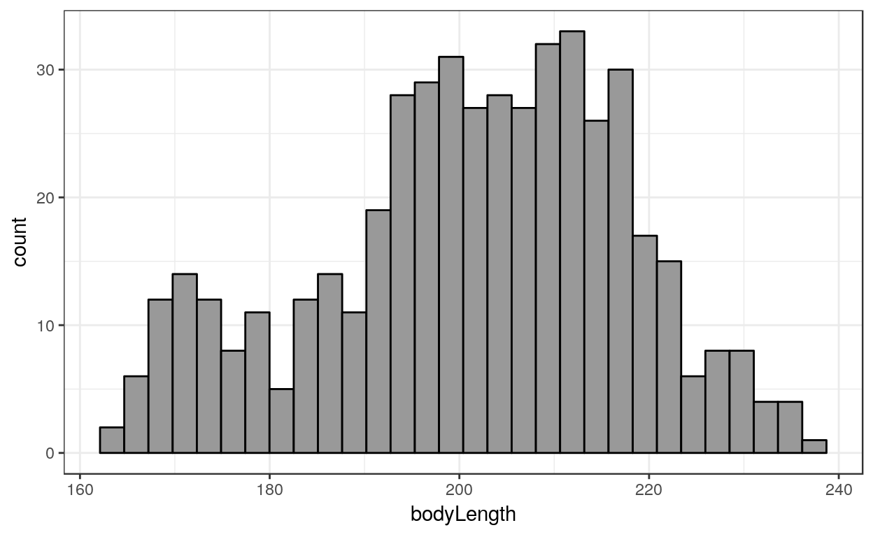
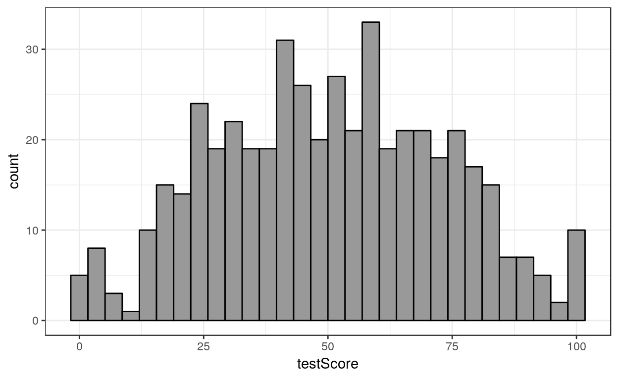
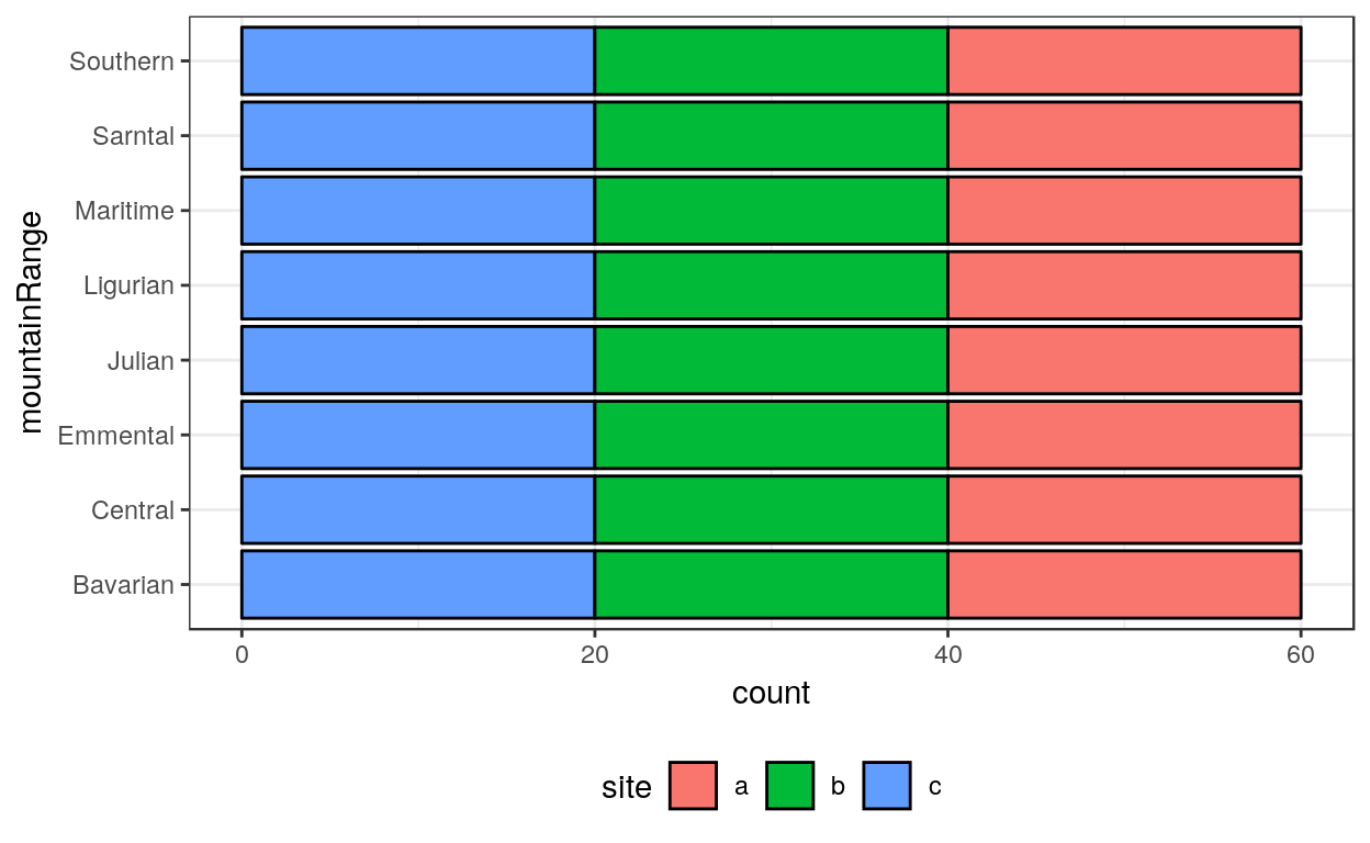
Statistiques univariées

Analyse statistique

Modèle linéaire simple

model_simple <- lm(testScore ~ bodyLength, data = dragons)

term	estimate	std.error	statistic	p.value
(Intercept)	-61.318	12.067	-5.081	0.000
bodyLength	0.555	0.060	9.287	0.000

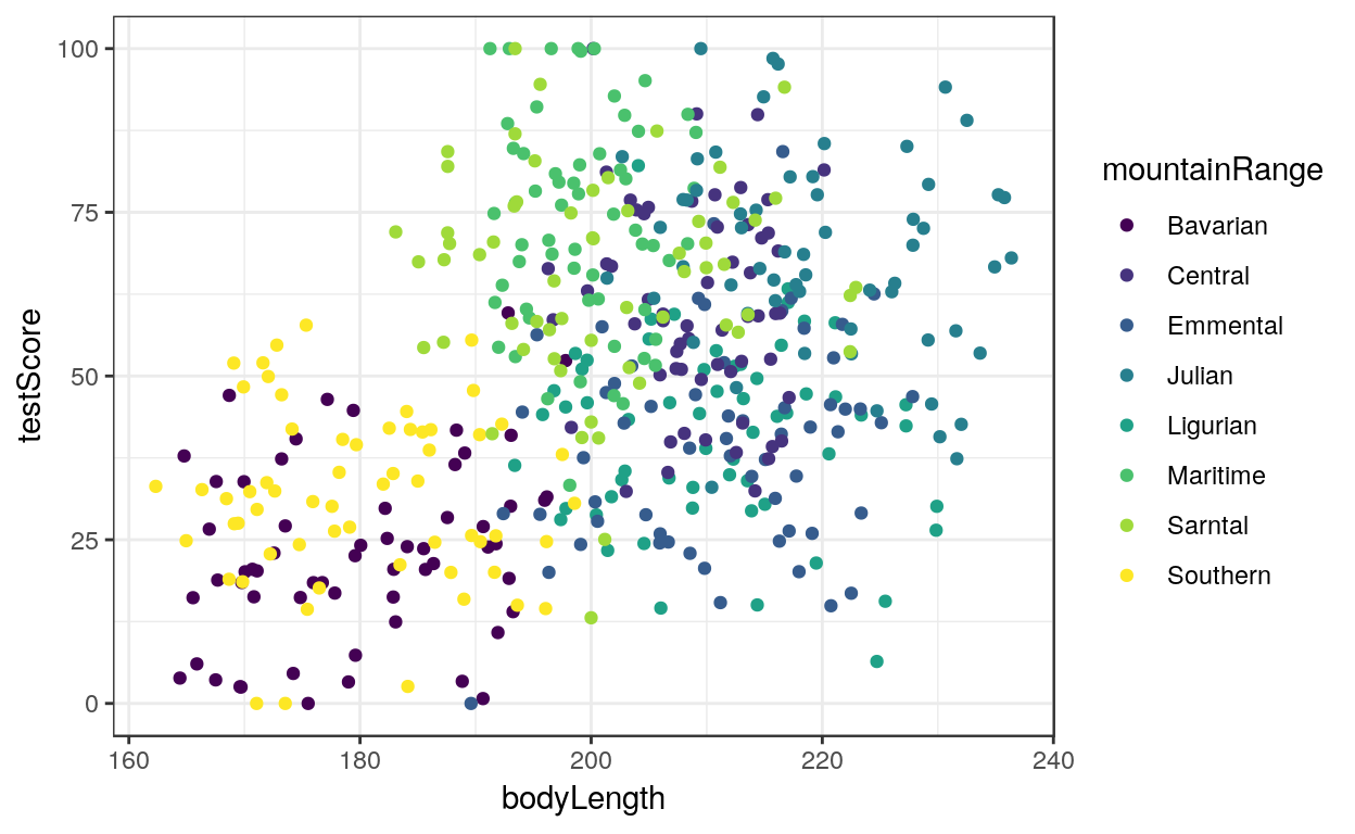
La longueur du dragon explique son intelligence.

ANCOVA

model_ancova <- lm(testScore ~ bodyLength + mountainRange, data = dragons)

On regarde les coefficients de chaque variable via broom::tidy().

term	estimate	std.error	statistic	p.value
(Intercept)	20.831	14.472	1.439	0.151
bodyLength	0.013	0.080	0.159	0.874
mountainRangeCentral	36.583	3.599	10.164	0.000
mountainRangeEmmental	16.209	3.697	4.385	0.000
mountainRangeJulian	45.115	4.190	10.767	0.000
mountainRangeLigurian	17.748	3.674	4.831	0.000
mountainRangeMaritime	49.881	3.139	15.890	0.000
mountainRangeSarntal	41.978	3.197	13.130	0.000
mountainRangeSouthern	8.520	2.731	3.119	0.002

On fait une analyse de la variance de type II via car::Ancova().

term	sumsq	df	statistic	p.value
bodyLength	5.653	1.000	0.025	0.874
mountainRange	109415.981	7.000	69.844	0.000
Residuals	105407.810	471.000

La longueur du dragon n’est plus significative pour expliquer son intelligence si on prend en compte la région d’où il vient.

Modèle mixte

On utilise le package lme4 pour faire du modèle mixte et broom.mixed pour mettre en forme les résultats.

library(lme4)
library(broom.mixed)

model_mixed <- lmer(testScore ~ bodyLength + (1|mountainRange), 
                    data = dragons, REML = TRUE)

On regarde tidy(model_mixed) et glance(model_mixed).

effect	group	term	estimate	std.error	statistic
fixed		(Intercept)	43.709	17.135	2.551
fixed		bodyLength	0.033	0.079	0.422
ran_pars	mountainRange	sd__(Intercept)	18.430
ran_pars	Residual	sd__Observation	14.960

sigma	logLik	AIC	BIC	REMLcrit	df.residual
14.960	-1995.601	3999.203	4015.898	3991.203	476

On va comparer ce modèle avec le modèle qui ne contient pas bodyLength.

model_mixed_null <- lmer(testScore ~ 1 + (1|mountainRange), 
                         data = dragons, REML = TRUE)

Puis on fait une anova de type I via anova().

term	df	AIC	BIC	logLik	deviance	statistic	Chi.Df	p.value
model_mixed_null	3.000	3999.685	4012.206	-1996.843	3993.685
model_mixed	4.000	4001.478	4018.173	-1996.739	3993.478	0.207	1.000	0.649

La variable n’est pas bodyLength n’est pas significative.

Modèle mixte à effets imbriqués

model_nested <- lmer(testScore ~ bodyLength + (1|mountainRange) + (1|mountainRange:site), 
                     data = dragons)

effect	group	term	estimate	std.error	statistic
fixed		(Intercept)	40.067	21.864	1.833
fixed		bodyLength	0.051	0.104	0.494
ran_pars	mountainRange:site	sd__(Intercept)	4.805
ran_pars	mountainRange	sd__(Intercept)	18.099
ran_pars	Residual	sd__Observation	14.442

sigma	logLik	AIC	BIC	REMLcrit	df.residual
14.442	-1987.980	3985.961	4006.830	3975.961	475

model_nested_null <- lmer(testScore ~ 1 + (1|mountainRange) + (1|mountainRange:site), 
                          data = dragons)

On fait une anova de type un entre model_nested et model_null.

term	df	AIC	BIC	logLik	deviance	statistic	Chi.Df	p.value
model_nested_null	4.000	3987.054	4003.749	-1989.527	3979.054
model_nested	5.000	3988.767	4009.636	-1989.384	3978.767	0.287	1.000	0.592

La modèle qui contient bodyLength n’est pas significativement différent du modèle qui ne le contient pas.

Notes

ML / REML

Par défaut, lmer() va optimiser REML et non pas ML. Cependant, lorsqu’on fait anova() entre deux modèles, ceux-ci sont recalculés pour être optimisés selon ML.

Prédiction

augment(model_nested, dragons)

# A tibble: 480 x 14
   testScore bodyLength mountainRange site  .fitted .resid .cooksd
       <dbl>      <dbl> <fct>         <fct>   <dbl>  <dbl>   <dbl>
 1     16.1        166. Bavarian      a        20.8  -4.62 2.38e-3
 2     33.9        168. Bavarian      a        20.9  13.0  1.82e-2
 3      6.04       166. Bavarian      a        20.8 -14.8  2.41e-2
 4     18.8        168. Bavarian      a        20.9  -2.04 4.47e-4
 5     33.9        170. Bavarian      a        21.0  12.9  1.73e-2
 6     47.0        169. Bavarian      a        20.9  26.1  7.21e-2
 7      2.56       170. Bavarian      a        21.0 -18.4  3.55e-2
 8      3.88       164. Bavarian      a        20.7 -16.8  3.24e-2
 9      3.60       168. Bavarian      a        20.9 -17.3  3.21e-2
10      7.36       180. Bavarian      a        21.5 -14.1  2.16e-2
# … with 470 more rows, and 7 more variables: .fixed <dbl>,
#   .mu <dbl>, .offset <dbl>, .sqrtXwt <dbl>, .sqrtrwt <dbl>,
#   .weights <dbl>, .wtres <dbl>

On a accès aux coefficients via les fonctions coefficients() pour les effets fixes et ranef() pour les effets aléatoires.

coefficients(summary(model_nested))

               Estimate Std. Error   t value
(Intercept) 40.06668990 21.8637329 1.8325640
bodyLength   0.05125931  0.1036824 0.4943879

ranef(model_nested)

$`mountainRange:site`
           (Intercept)
Bavarian:a -2.46727186
Bavarian:b -3.05278205
Bavarian:c  3.73563393
Central:a  -6.38640673
Central:b   0.84540907
Central:c   6.17300851
Emmental:a -3.02659531
Emmental:b  2.29768424
Emmental:c -0.03273939
Julian:a    2.42006432
Julian:b    2.20653961
Julian:c   -3.44048746
Ligurian:a  0.99876698
Ligurian:b -0.84624351
Ligurian:c -0.80816294
Maritime:a -3.67613987
Maritime:b -0.63034574
Maritime:c  5.87130429
Sarntal:a   3.65403344
Sarntal:b  -4.91065013
Sarntal:c   2.27894013
Southern:a -0.68072360
Southern:b  2.18570243
Southern:c -2.70853837

$mountainRange
         (Intercept)
Bavarian  -25.313507
Central     8.965609
Emmental  -10.804656
Julian     16.826066
Ligurian   -9.300801
Maritime   22.198277
Sarntal    14.502523
Southern  -17.073511

La prédiction se fait en additionnant les différentes composantes.

# Ordonné à l'origine
coefficients(summary(model_nested))[1, 1] + 
  # Taille des 6 premiers dragons * coefficient de cette variable
  dragons$bodyLength[1:6] * coefficients(summary(model_nested))[2, 1] +
  # Coefficient dû à la montagne (Bavarian pour les 6 premiers)
  ranef(model_nested)$mountainRange["Bavarian", ] +
  # Coefficient dû au site dans la montagne (Bavarian:a pour les 6 premiers)
  ranef(model_nested)$`mountainRange:site`["Bavarian:a", ]

[1] 20.77181 20.87488 20.78896 20.88135 20.99793 20.93278

Et on retrouve le même résultat

augment(model_nested, dragons)$.fitted[1:6]

[1] 20.77181 20.87488 20.78896 20.88135 20.99793 20.93278

Probabilités critiques

Si veut les probabilités critiques pour chaque variable, on a besoin de charger le package lmerTest.

library(lmerTest)

model_mixed <- lmer(testScore ~ bodyLength + (1|mountainRange), 
                    data = dragons)

effect	group	term	estimate	std.error	statistic	df	p.value
fixed		(Intercept)	43.709	17.135	2.551	177.466	0.012
fixed		bodyLength	0.033	0.079	0.422	472.667	0.673
ran_pars	mountainRange	sd__(Intercept)	18.430
ran_pars	Residual	sd__Observation	14.960

sigma	logLik	AIC	BIC	REMLcrit	df.residual
14.960	-1995.601	3999.203	4015.898	3991.203	476

La variable bodyLength n’est pas significative.

Conclusion

On a un joli paradoxe de Simpson :)